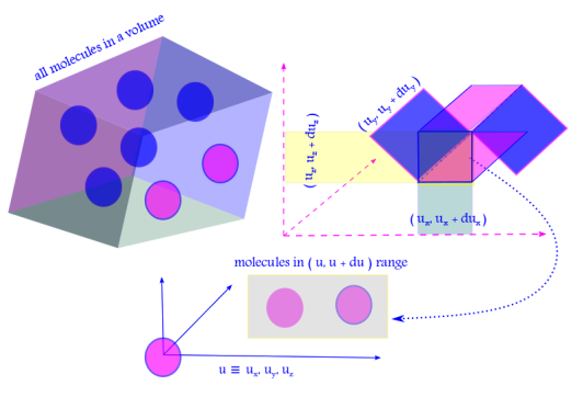
i. We assume a dilute gas which is enclosed by a thermally insulated container on all sides.
Maxwell Boltzmann Distribution: dilute gas in a thermally insulated container: dilute means concentration of gas molecules is low, insulated implies there is no reasonable flow of heat energy across the walls of the container. Photo Credit: mdashf.org
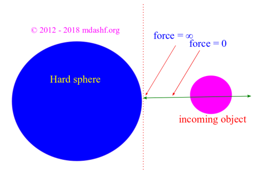
ii. Each molecule is assumed to be a hard sphere which moves randomly in all directions such that its velocity varies from .
Maxwell Boltzmann Distribution: Hard sphere; remember a hard sphere is a classical analogy of a rigid sphere whose surfaces do not deform when an external object comes into contact. This essentially means the incoming object is scattered elastically that is without loss of kinetic energy, only momenta magnitude and directions are changed in accordance with the conservation of linear momentum. Photo Credit: mdashf.org
iii. When molecules collide they do not lose energy or time. They bounce off each other so that ‘energy‘ and ‘momenta‘ are conserved.
Maxwell Boltzmann Distribution: Ideal gas molecules; the collision of molecules have been assumed to be elastic scattering of hard sphere. The process occurs instantaneously without wasting molecules hard-pressed professional time. They just meet, talk no non-sense, exchange any energy or momenta and move on. As a consequence energy and momenta are conserved. Photo-Credit: mdashf.org
iv. We would like to obtain an expression for velocity distribution function. That is we would like to know the fraction of molecules having velocity between for all possible values of velocity.
For this we assume an ensemble of molecules in equilibrium. The ratio of number of molecules in a velocity range to the total number of molecules N gives the probability of finding a molecule in that velocity range.
v. The “phase space” of the ensemble of molecules is defined by a 6 N dimensional space, which constitutes of 3 N spatial components and 3 N velocity components of the N molecules in equilibrium. For a more advanced concept of phase space check the following statistical mechanics lecture.
vi. is the probability that a given molecule is found to have its x component of velocity in the range .
Maxwell Boltzmann Distribution Probability function: number of molecules with a specified value of velocity ( eg having x component of velocity in a given window of values ) corresponds to a probability function defined for the same. eg We can define 3 different probability functions fx, fy and fz for likelihood of finding a molecule exclusively for a given axis of velocity vector. Photo-Credit: mdashf.org
Similarly and give the probability that a molecule would have its y-component of velocity in the window of and z-component of velocity in the window of respectively.
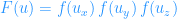
vii. The x, y and z components of the velocities are considered to be independent of each other. The probability that a molecule will simultaneously have its x-component of velocity in the window , y-component of velocity in the window and z-component of velocity in the window is given by .
Maxwell Boltzmann Distribution: A 3 dimensional probability function gives the likelihood of finding a molecule simultaneously with 3 exclusive values for the 3 components of velocities. Photo-Credit: mdashf.org
This follows from the law of probability of mutually exclusive events, happening all at once.
viii. The total number of molecules in the phase space is thus: . If the velocity of a molecule is , so the magnitude is then is the joint probability density ( or distribution function ) for the molecule to be found with velocity .
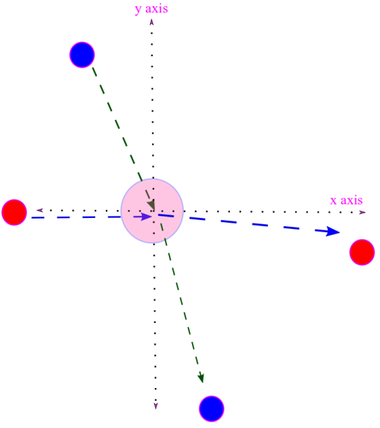
F(u) is a radial function, i.e. independent of angular variables defined by x, y, z components of the velocity vector with x, y, z axes. This isotropic nature of velocity follows from the lack of a “favored direction” due to random motion of the molecules.
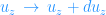
ix. From we can write or . This is because since does not change to first order, when make infinitesimal changes.
Note that the prime denotes differentiation wrt the argument of the function ( i.e. any variable inside the parenthesis dictating values to the function itself ).
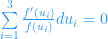
x. Lets divide the previously obtained equation ( in ix. ) by the factor: . We obtain: . We can write this concisely as a summation over a repeated index as is customary. We have ( you can quote this to your mother in law, she wouldn’t disagree );
.
xi. The magnitude of the measured velocity ( ) must remain unchanged. Hence ⇒⇒, again this can be written concisely ( and presented to difficult people to please them )
We have; .
We can multiple this by a Lagrange multiplier ( constant ) B and add to equation obtained in x.
xii. We obtain;
The infinitesimal changes in x, y and z components of velocities, i.e. are non-zero and independent of each other.
⇒.
B is a constant which needs to be determined from physical conditions on the system.
xiii. If we solve the differential equation in xii, we obtain here C is a constant which also needs to be determined to get . We have after toiling through all the above exercises: .
Evaluation of constants B and C
i. Constant C: Lets evaluate C in terms of B. This is achieved the by the “condition of normalization“. Since a particular gas molecule must be found somewhere in the container of volume V, the probability function F(u) integrated over all of phase space and over entire volume V must give V. ⇒ ⇒ or . This gives . Usefulness of gamma function for evaluating integrals: This was achieved by using the results of integration by the method of gamma function, which will be linked when its available on the website. Its intended as a homework at the moment. Homework: show by the method of Γ function that we already discussed ( in the mathematical physics lectures, that will be available in the website in due time ) the following. . This would mean and .
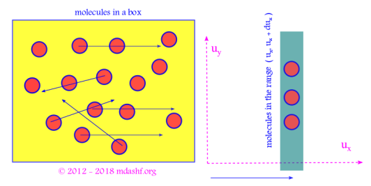
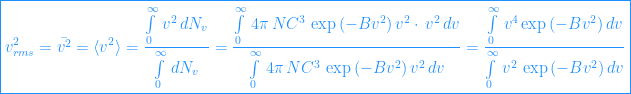
ii. Constant B: We need to evaluate the root-mean-square velocity in order for us to be able to obtain B. Lets do that. “We use here the idea of taking average of any quantity, which is a pretty basic concept and we will meet time and again, in many different areas of physics. Since we are doing it over the distribution of velocities of the molecules it is given by the following definition.” . Gamma function: the two integrals are solved by the same Γ function method we used ( with the aid of the home work ) above. The result is: . Probability density and number denisty of molecules, in a particular velocity range: here we have used the following: the first expression is a probability density that we derived in xiii and the second one is its application, the absolute number of molecules in a window of velocity obtained by multiplying this probability f(ux) by the total number of molecules in our sample N. This is just for one dimension ( x here ) To find the number in the infinitesimal volume surrounding a given velocity value we simply multiply the corresponding expressions for each dimension, so; . Note that the probabilities are multiplied first then the total number of molecules N is multiplied to the 3 dimensional probability density only once, so we do not have N3 but N. Neither do we have a cubic power in the exponential function, for the same reason. We define the number density ( ) as the number of molecules in a unit velocity window surrounding the value of a given velocity , it is given by . When we said unit we meant we needed to divide by any arbitrary value of window of velocity to make it unit, this arbitrary value of window of velocity here is the infinitesimal volume element with value: .
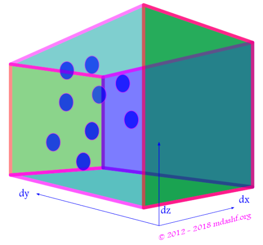
Maxwell Boltzmann Distribution: Molecules in an infinitesimal box of volume dx-dy-dz obtained by multiplying probability density with total number of molecules. Photo-Credit: mdashf.org
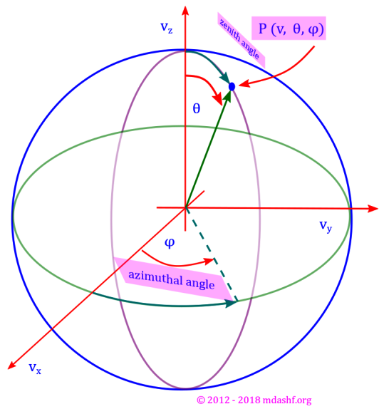
( a ) Usefulness of spherical polar coordinate system: “In viii we noted that our gas sample is isotropic in nature, which means our velocity distribution probability function ( F ) is not dependent on velocity direction but only on its magnitude. This is due to the fact that the gas molecules have random motion.” Due to this reason it becomes quite less involved to work in the spherical polar coordinate system. At the moment we are not going to the nitty gritties of this system of coordinate, but rather use its basic results. If and when any helpful material from my other lectures is available it would be linked. We will use couple of diagrams which would help us visualize the variables we are using. Note that the images use the system in terms of position coordinates ( ) but we want to employ the system for velocity vector, so for our purpose it suffices to redefine r by u, the magnitude of the position vector by the magnitude of the velocity vector. Similarly ( ) must be redefined as ( ). The angles ( ) remain the same. Number of molecules in an infinitesimal volume: with the above in the spherical polar coordinate system the number of molecules in any volume is obtained by multiplying the volume with number density as defined above, so we have . Note that we did not do an integration performed over the magnitude of the velocity vector because we need to study the probability or distribution over this variable. So we have: . This is in-fact the result we have used in derivation of constant B above in ii. With all this exercise we got an expression for constant B in terms of the average of the square of velocity magnitude over all possible values for our sample.
Maxwell Boltzmann Distribution: Spherical polar coordinates: azimuth angle ( φ ) zenith angle ( θ ) and vector magnitude variable (radial component, here v) where v, θ and φ are related to vx, vy and vz by: vx = v sin θ cos φ, vy = v sin θ sin φ and vz = v cos θ. We shall also note that functions that are spherically symmetric do not depend upon angular dimensions, in other words they are independent of θ and φ. Photo-Credit: mdashf.org
( b ) Usefulness of equipartition energy theorem: This is useful since we can relate the distribution ( of speed ) to the temperature of the gas sample by the profound result known as equipartition energy theorem which we will have opportunities to derive later in this series and in our statistical mechanics series. When they are available in other lectures of mine, I will link them here. ( We can also derive the same using the result that we will obtain soon, but thats a circular logic like a website back and forward button ). The equipartition energy theorem states that each degree of freedom of a kinetic system ( such as the one we are discussing with our hard sphere assumption and elastic scattering ) has on an average the kinetic energy per molecule given by: where the kB is the Boltzmann constant. This helps us obtain a value of B in terms of absolute temperature T. ⇒ and consequently . Finally we can write the Maxwell Boltzmann velocity distribution function. Note that the following expression gives the absolute number of molecules dNu in the volume element surrounding the value of a given velocity magnitude u. If one divides the total number of molecules N, one would get the probability in a velocity range du. Further dividing du one would get the probability density of finding the molecules at a given value of magnitude of velocity vector u, which would be the function of the same, the probability function f would be a function of u that is. Maxwell Boltzmann velocity distribution for an ideal gas: .
“Maxwell Boltzmann distribution function for speed and energy, rms, average and most probable values for speed and energy”
Lectures III — IV
We derived a relation for distribution of molecular speed of an ideal gas which we called the Maxwell Boltzmann distribution. It is given as follows.
Here dNv is the number of molecules having speed within v → v + dv. Note that we have reverted back to a regular symbol v, for velocity. One should be comfortable doing that in physics. N is the total number of molecules in the ensemble we considered. kB is the Boltzmann constant whose value is given as kB = 1.38×10⁻²³ J/K. m is the mass of the molecule.
We call as the Maxwell Boltzmann distribution function. It is a probability density function ( often called in short pdf , not to confound with portable document format though) or distribution for finding the molecule in the speed range of v and v + dv.
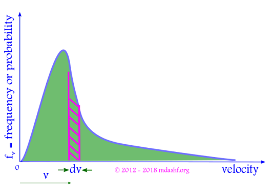
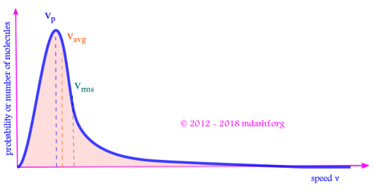
Maxwell Boltzmann Distribution: The Maxwell Boltzmann probability density function shows likelihood of finding a molecule in a given velocity ( speed ) range. Photo-Credit: mdashf.org
Properties of Maxwell Boltzmann probability function
i. The shape of the function is an increasing quadratic function ( due to v2 ) and a decreasing exponential function.
ii. is the area under the curve between velocities v and v + dv, shown as the shaded portion in the figure above. It gives the number of molecules within velocity v to v + dv.
iii. The total area under the curve is 1, as its a true probability distribution. This is same as the condition of normalization.
iv. The increasing quadratic function dominates for small values of velocity v. For larger velocities exponential function dominates and the curve begins to fall. The curve is asymmetric.
v. The probability fvis zerofor two values of velocity, v = 0and v = ∞. That means molecules can travel only at finite and non-zero speeds.
vi. The probability function fv has a peak. It corresponds to a velocity where maximum number of molecules are found. Consequently this value of the velocity for which there is a peak in the probability distribution is known as “most probable velocity” and denoted as vmp or vp.
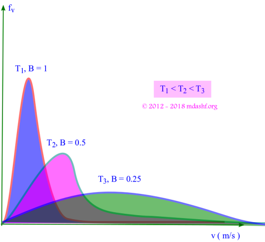
vii. As Tincreases B decreases since B = m/2kBT. The curve becomes flatter, the peak is reduced and the curve shifts to right. This causes the molecules to become more energetic.
Maxwell Boltzmann Distribution: The behavior of Maxwell Boltzmann velocity distribution with increasing temperature. Photo Credit: mdashf.org
Mean, rms and most probable speed
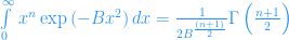
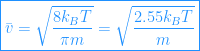
a.Mean or average speed : As we have already seen the mean of variable for which a functional distribution exists can be given as follows. . ⇒. The integral is in terms of Γ function. We have already done this a few times. We will use the same formula as follows for n = 3. . So we have; . We know that Γ( 2 ) = 1. With this we get the expression for the average value for the velocity of a group f molecules in a sample of container with ideal gas assumptions. . This gives the final expression for the average speed. We obtain the average speed: .
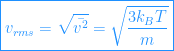
b. Root-mean-square or rms speed: RMS speed is defined as ( we have seen this above while evaluating our constants B and C ) i.e. the square root of the mean of the speed-squared. We have already evaluated the integral for and we found where . So . Thus we obtain for the rms speed: .
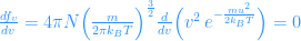
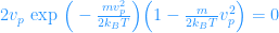
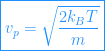
c. Most probable speed: The most probable speed is the speed at which Maxwell’s probability function shows a peak. At this point first derivative of fv wrt v is zero and its second derivative is negative. ⇒. The value of v where the first derivative is zero is vp and so ⇒. Since ⇒ or . This give the most probable speed. Thus we obtain the most probable speed: . It can be easily shown that at v = vp; . Thus fv has a peak or maxima indeed at the most probable speed value vp.
From the 3 expressions for the 3 kinds of speeds we see that: vrms > vav > vp.
Maxwell Boltzmann Distribution for velocity: There is a strict relationship among the most probable, rms and mean speed in a Maxwell Boltzmann distribution of velocities for a classical ideal gas. Photo Credit: mdashf.org
Maxwell Boltzmann distribution for energy
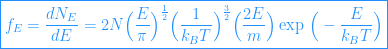
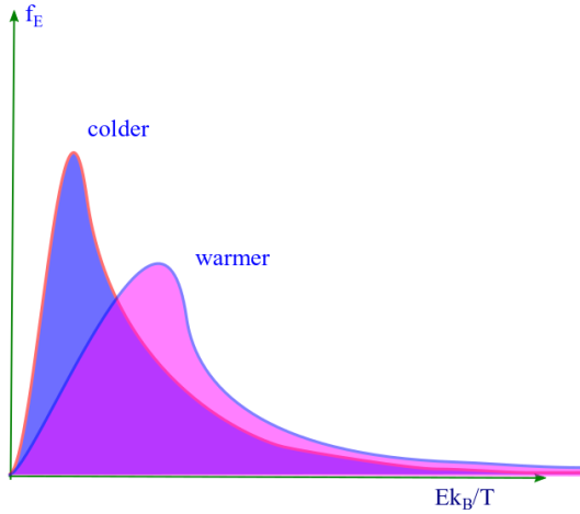
Maxwellian energy distribution. We studied in much detail the distribution of velocity of molecules in a classical ideal gas according to the Maxwell Boltzmann distribution. We can use the same to cast it into a form which depicts the energy behavior of the molecules. We had . We would call the energy distribution function as the Maxwell Boltzmann energy distribution function ( or in short Maxwellian energy distribution ) and denote it as fE. For the ideal gas molecule of mass m, and speed v its kinetic energy is given by: E = 1/2 mv2. So that dE = mvdv or . Also . The number of molecules found in the speed range v to v + dv is also same as the number of molecules found in the energy range E to E + dE. This is stated by the simple expression: dNE = dNv. From the expression for velocity distribution written above, we have: . Simplifying . From this the energy distribution function is given by: . At a given temperature energy distribution function fE is a product of square root of energy ( √E ) and a decreasing or decaying exponential. A plot of fE vs E/kBT is shown. The peak in the distribution function ( fE ) suggests that there is a most probable energy ( Ep ) at which there is a likelihood of finding the highest number of molecules than at any other energy. Similarly we can find the mean or average energy of the distribution ( Eav= ).
The Maxwell Boltzmann Distribution for energy: probability vs energy ( at a fixed temperature ) for two different temperatures. Photo Credit: mdashf.org
Lets find these two values.
Mean and most probable energy
a. Mean or average energy of Maxwellian gas: Mean energy of a molecule in a Maxwellian gas is defined as: . Simplifying this we get: . If x = E/kBT then dx = (kBT)-1dE, then; . This leads us to obtain average energy: .
b. Most probable energy of Maxwellian gas: Most probable energy is that energy E= Epfor which ( and ). So or . Thus we obtain the most probable energy: .
i. Mean vs most probable energy
Mean energy of a Maxwellian gas ( ) is 3 times the most probable energy ( ). i.e. .
ii. Mean energy at a fixed temperature
At a given temperature mean energy is same for all gases, irrespective of their nature e.g. at room temperature ( T = 300 K ) or .
iii. Momentum distribution function
The number of molecules with momentum within p to p + dp is given by .
This finishes our 4 lecture hours of concepts on Maxwell Boltzmann distribution function. This will be followed by 4 lecture hours of 13 solved examples and numerical. Its hoped this will come pretty soon.


![d[f(u_x)\,f(u_y)\,f(u_z)] \, =\,dF(u)](https://s0.wp.com/latex.php?latex=d%5Bf%28u_x%29%5C%2Cf%28u_y%29%5C%2Cf%28u_z%29%5D+%5C%2C+%3D%5C%2CdF%28u%29+&bg=ffffff&fg=1e90ff&s=0&c=20201002)
![[f'(u_x)\,du_x]f(u_y)f(u_z)+ [f'(u_y)\,du_y]f(u_x)f(u_z)+[f'(u_z)\,du_z]f(u_x)f(u_y)=0](https://s0.wp.com/latex.php?latex=%5Bf%27%28u_x%29%5C%2Cdu_x%5Df%28u_y%29f%28u_z%29%2B+%5Bf%27%28u_y%29%5C%2Cdu_y%5Df%28u_x%29f%28u_z%29%2B%5Bf%27%28u_z%29%5C%2Cdu_z%5Df%28u_x%29f%28u_y%29%3D0&bg=ffffff&fg=1e90ff&s=0&c=20201002)


![d[u_x^2+u_y^2+u_z^2]=d[u^2]=0](https://s0.wp.com/latex.php?latex=d%5Bu_x%5E2%2Bu_y%5E2%2Bu_z%5E2%5D%3Dd%5Bu%5E2%5D%3D0&bg=ffffff&fg=1e90ff&s=0&c=20201002)


![\sum\limits_{i=1}^{3}\Big[\frac{f'(u_i)}{f(u_i)}\,+\,B\,u_i\Big]\,du_i](https://s0.wp.com/latex.php?latex=%5Csum%5Climits_%7Bi%3D1%7D%5E%7B3%7D%5CBig%5B%5Cfrac%7Bf%27%28u_i%29%7D%7Bf%28u_i%29%7D%5C%2C%2B%5C%2CB%5C%2Cu_i%5CBig%5D%5C%2Cdu_i+&bg=ffffff&fg=1e90ff&s=0&c=20201002)


![\boxed{F(u)=f(u_x)\,f(u_y)\,f(u_z)=C^3\exp\,[-B(u_x^2+u_y^2+u_z^2)]}](https://s0.wp.com/latex.php?latex=%5Cboxed%7BF%28u%29%3Df%28u_x%29%5C%2Cf%28u_y%29%5C%2Cf%28u_z%29%3DC%5E3%5Cexp%5C%2C%5B-B%28u_x%5E2%2Bu_y%5E2%2Bu_z%5E2%29%5D%7D&bg=ffffff&fg=1e90ff&s=0&c=20201002)

![\boxed{\Bigg[C\,\int\limits_{-\infty}^{\infty}\,du_x\,\exp\,(-B\,u_x^2)\Bigg]^3=1}](https://s0.wp.com/latex.php?latex=%5Cboxed%7B%5CBigg%5BC%5C%2C%5Cint%5Climits_%7B-%5Cinfty%7D%5E%7B%5Cinfty%7D%5C%2Cdu_x%5C%2C%5Cexp%5C%2C%28-B%5C%2Cu_x%5E2%29%5CBigg%5D%5E3%3D1%7D+&bg=ffffff&fg=1e90ff&s=0&c=20201002)


![\boxed{\langle v^2 \rangle = {\frac{1}{2B^{\frac{5}{2}}}\,\Gamma\,\Big(\,\frac{5}{2}\,\Big)}\times \bigg[{\frac{1}{2B^{\frac{3}{2}}}\,\Gamma\,\Big(\,\frac{3}{2}\,\Big)}\bigg]^{-1} =\frac{3}{2B}}](https://s0.wp.com/latex.php?latex=%5Cboxed%7B%5Clangle+v%5E2+%5Crangle+%3D+%7B%5Cfrac%7B1%7D%7B2B%5E%7B%5Cfrac%7B5%7D%7B2%7D%7D%7D%5C%2C%5CGamma%5C%2C%5CBig%28%5C%2C%5Cfrac%7B5%7D%7B2%7D%5C%2C%5CBig%29%7D%5Ctimes+%5Cbigg%5B%7B%5Cfrac%7B1%7D%7B2B%5E%7B%5Cfrac%7B3%7D%7B2%7D%7D%7D%5C%2C%5CGamma%5C%2C%5CBig%28%5C%2C%5Cfrac%7B3%7D%7B2%7D%5C%2C%5CBig%29%7D%5Cbigg%5D%5E%7B-1%7D+%3D%5Cfrac%7B3%7D%7B2B%7D%7D&bg=ffffff&fg=1e90ff&s=0&c=20201002)


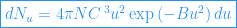


![\boxed{dN_u=4\pi N \bigg(\frac{m}{2\pi k_B T}\bigg)^\frac{3}{2}u^2\exp \,\Big[-\Big(\frac{mu^2}{2k_B T}\Big)\Big]du}](https://s0.wp.com/latex.php?latex=%5Cboxed%7BdN_u%3D4%5Cpi+N+%5Cbigg%28%5Cfrac%7Bm%7D%7B2%5Cpi+k_B+T%7D%5Cbigg%29%5E%5Cfrac%7B3%7D%7B2%7Du%5E2%5Cexp+%5C%2C%5CBig%5B-%5CBig%28%5Cfrac%7Bmu%5E2%7D%7B2k_B+T%7D%5CBig%29%5CBig%5Ddu%7D+&bg=ffffff&fg=1e90ff&s=0&c=20201002)
![dN_v=4\pi N \big(\frac{m}{2\pi k_B T}\big)^\frac{3}{2}v^2\exp\,\Big[-\Big( \frac{mv^2}{2k_B T} \Big) \Big]dv](https://s0.wp.com/latex.php?latex=dN_v%3D4%5Cpi+N+%5Cbig%28%5Cfrac%7Bm%7D%7B2%5Cpi+k_B+T%7D%5Cbig%29%5E%5Cfrac%7B3%7D%7B2%7Dv%5E2%5Cexp%5C%2C%5CBig%5B-%5CBig%28+%5Cfrac%7Bmv%5E2%7D%7B2k_B+T%7D+%5CBig%29+%5CBig%5Ddv+&bg=ffffff&fg=1e90ff&s=0&c=20201002)


![dN_v=4\pi N \big(\frac{m}{2\pi k_B T}\big)^\frac{3}{2}v^2\exp\,\Big[-\Big( \frac{mu^2}{2k_B T} \Big) \Big]dv](https://s0.wp.com/latex.php?latex=dN_v%3D4%5Cpi+N+%5Cbig%28%5Cfrac%7Bm%7D%7B2%5Cpi+k_B+T%7D%5Cbig%29%5E%5Cfrac%7B3%7D%7B2%7Dv%5E2%5Cexp%5C%2C%5CBig%5B-%5CBig%28+%5Cfrac%7Bmu%5E2%7D%7B2k_B+T%7D+%5CBig%29+%5CBig%5Ddv+&bg=ffffff&fg=1e90ff&s=0&c=20201002)
![\bar{v}=\frac{1}{N}\times 4\pi N \big(\frac{m}{2\pi k_B T}\big)^\frac{3}{2}\int\limits_{0}^{\infty}\,v^3\exp\,\Big[-\Big( \frac{mu^2}{2k_B T} \Big) \Big]dv](https://s0.wp.com/latex.php?latex=%5Cbar%7Bv%7D%3D%5Cfrac%7B1%7D%7BN%7D%5Ctimes+4%5Cpi+N+%5Cbig%28%5Cfrac%7Bm%7D%7B2%5Cpi+k_B+T%7D%5Cbig%29%5E%5Cfrac%7B3%7D%7B2%7D%5Cint%5Climits_%7B0%7D%5E%7B%5Cinfty%7D%5C%2Cv%5E3%5Cexp%5C%2C%5CBig%5B-%5CBig%28+%5Cfrac%7Bmu%5E2%7D%7B2k_B+T%7D+%5CBig%29+%5CBig%5Ddv+&bg=ffffff&fg=1e90ff&s=0&c=20201002)
![\int\limits_{0}^{\infty}\,v^3\exp\Big[-\Big( \frac{mu^2}{2k_B T} \Big) \Big]dv=\frac{1}{2\big( \frac{m}{2k_B T} \big)^2}\,\Gamma(2)](https://s0.wp.com/latex.php?latex=%5Cint%5Climits_%7B0%7D%5E%7B%5Cinfty%7D%5C%2Cv%5E3%5Cexp%5CBig%5B-%5CBig%28+%5Cfrac%7Bmu%5E2%7D%7B2k_B+T%7D+%5CBig%29+%5CBig%5Ddv%3D%5Cfrac%7B1%7D%7B2%5Cbig%28+%5Cfrac%7Bm%7D%7B2k_B+T%7D+%5Cbig%29%5E2%7D%5C%2C%5CGamma%282%29&bg=ffffff&fg=1e90ff&s=0&c=20201002)
![\bar{v}=4\pi \big(\frac{m}{2\pi k_B T}\big)^{\frac{3}{2}}\big[\big(\frac{m}{2k_B T}\big)^2\big]^{-1} =\sqrt{\frac{8k_B T}{\pi m}}](https://s0.wp.com/latex.php?latex=%5Cbar%7Bv%7D%3D4%5Cpi+%5Cbig%28%5Cfrac%7Bm%7D%7B2%5Cpi+k_B+T%7D%5Cbig%29%5E%7B%5Cfrac%7B3%7D%7B2%7D%7D%5Cbig%5B%5Cbig%28%5Cfrac%7Bm%7D%7B2k_B+T%7D%5Cbig%29%5E2%5Cbig%5D%5E%7B-1%7D+%3D%5Csqrt%7B%5Cfrac%7B8k_B+T%7D%7B%5Cpi+m%7D%7D+&bg=ffffff&fg=1e90ff&s=0&c=20201002)


![const \times [2v\,\exp\,(-Bv^2)+v^2\,\exp\,(-Bv^2)\times \big(\frac{-2mv}{2k_B T}\big)]=0](https://s0.wp.com/latex.php?latex=const+%5Ctimes+%5B2v%5C%2C%5Cexp%5C%2C%28-Bv%5E2%29%2Bv%5E2%5C%2C%5Cexp%5C%2C%28-Bv%5E2%29%5Ctimes+%5Cbig%28%5Cfrac%7B-2mv%7D%7B2k_B+T%7D%5Cbig%29%5D%3D0+&bg=ffffff&fg=1e90ff&s=0&c=20201002)


![\frac{d}{dE}\big[\sqrt{E}\exp\big(-\frac{E}{k_B T}\big)\big]\Big|_{E=E_p}=0](https://s0.wp.com/latex.php?latex=%5Cfrac%7Bd%7D%7BdE%7D%5Cbig%5B%5Csqrt%7BE%7D%5Cexp%5Cbig%28-%5Cfrac%7BE%7D%7Bk_B+T%7D%5Cbig%29%5Cbig%5D%5CBig%7C_%7BE%3DE_p%7D%3D0+&bg=ffffff&fg=1e90ff&s=0&c=20201002)
![\Big[\frac{1}{2\sqrt{E_p}}-\frac{\sqrt{E_p}}{k_B T}\Big]exp\,\Big(-\frac{E_p}{k_B T}\Big) =0](https://s0.wp.com/latex.php?latex=%5CBig%5B%5Cfrac%7B1%7D%7B2%5Csqrt%7BE_p%7D%7D-%5Cfrac%7B%5Csqrt%7BE_p%7D%7D%7Bk_B+T%7D%5CBig%5Dexp%5C%2C%5CBig%28-%5Cfrac%7BE_p%7D%7Bk_B+T%7D%5CBig%29+%3D0+&bg=ffffff&fg=1e90ff&s=0&c=20201002)

) is 3 times the most probable energy (
). i.e.
.
or
.
.

Leave a comment