Conductivity and mobility in semiconductors, L-III

Analog systems and applications, lecture — III

“Semiconductors: Conductivity and Mobility.”

This article belongs to a series of lectures on analog electronics, the paper goes by the name “Analog Systems and Applications” for the physics honors degree class. All lectures of this series will be found here. This is the third lecture of this series. This particular lecture was delivered on 8th January 2018.

We will discuss in this lecture about drift velocity of electrons and holes in semiconductors which leads to the conductivity and mobility of free charge carriers in the same.

To smooth-sail through this lecture you might wanna first brush up the concepts discussed in the last two lectures: lecture I and lecture II.

Lets begin with Ohm’s law: I=V/R. — eqⁿ 1

Here I is the electric current, V is the applied potential difference and R is the resistance of the material considered. The resistance R depends upon the length l and area of cross-section A of the given material. Let us cast Ohm’s law into a form which is independent of l and A.

For this we define electric current density J which is electric current per unit area (rate of charge flow perpendicularly across an area): J=I/A.

We know that the resistance of a piece of material is given by: R=ρL/A, where ρ is known as the “resistivity” of the given material, it is the resistance of a material of a unit length and unit cross-sectional area.

We also know that if an electric field E exists across length L of the material then its potential difference V is given by: E=V/L. If we define “electric conductivity” (σ) of the material as the reciprocal of its resistivity then; σ=1/ρ and Ohm’s law becomes: J=σE — eqⁿ 2.

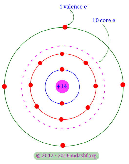
According to the free electron gas model it is the conduction electrons which are essentially free to move in the material and responsible for carrying the electric current. The ions which also consist of the non-conduction electrons (inner electrons or electrons in the core of the semiconductor as we have discussed in earlier lectures of this series) are not mobile. They are attached about the “lattice points”, in equilibrium condition.

When an external field E is applied across the material the conduction electrons experience two forces;

i. force due to electric field: -eE.

ii. frictional force due to collision of electrons with the rest of the medium: -m*v/τ.

Here m* is the “effective mass” of the electrons. m* is different from the actual electronic mass m₀ in general. m* arises from interaction of the electron in the lattice.

v is the velocity with which the electron moves and τ is known as “relaxation time” or “collision time“. It is the time on an average between successive collision. It gives the “probability” that an electron will undergo collision.

Note i: 1/τ is the frequency of collision and probability is proportional to the frequency, hence 1/τ.

Note ii: frictional force bears an impulse-momentum relation as given by, f=-m*v/τ.

We can now write the equation of motion for the electron: 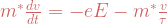. — eqⁿ 3

Collision would gradually reduce velocity to zero. But due to applied external force through E (or V), we reach a constant terminal velocity. This velocity is known as “steady state velocity“. At equilibrium: .

Thus at equilibrium we obtain this steady state velocity, given as: . — eqⁿ 4

i. v in eqⁿ 4 above is known as “drift velocity“. It is directed opposite to the electric field E and is denoted by v_d.

ii. v=v_r is the random velocity of the electron.

v_r >> v The random velocity is far larger than the drift velocity. it does not contribute to the electric current though, and therefore it has got no roles to play in the conductivity σ.

The drift velocity is given by — eqⁿ 4; .

Let there be N electrons per unit volume (in the material). N is also known as “electron concentration“. Net charge is then given by: -Ne. It then follows that there are number of conduction or free electrons. Z_v is the valence electrons per atom. ρ_m is the density of mass. N_A is the Avogadro number and M’ is the molar mass of the material element.

Now current density J is given by “total charge” into drift velocity (consider a cylinder of unit area of cross-section and length v_d per unit time). The idea behind what is current density is given in this article. (Current density)

Then; J=(-Ne)v_d=(-Ne)(-eτE/m*)=Ne²τE/m*. Then current density is given by: 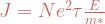. — eqⁿ 5

Conductivity is thus (from Ohm’s law that we derived in the beginning) σ=J/E. or: . — eqⁿ 6.

τ can be written in terms of “mean free path” ( l or λ ). It is the distance on an average covered by the electron between successive collisions. Mean free time is then given as: τ=l/v_r.

So conductivity can also be written as: 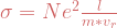. — eqⁿ 7.

Power dissipated is also power absorbed by the electrons (from the applied field). So, P=NFv_d=N(-eE)(-eτE/m*). Consequently: 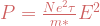. — eqⁿ 8.

We can write for the electron (majority carrier in n-type semiconductors); . — eqⁿ 9.

There are about N=10¹⁵/cm³=10²¹/m³ electrons in a semiconductor. τ is of the order of 10^-12 s. Electron effective mass is m_e = 0.1 m₀. Then σ_e ≅ 1 (ohm-m)^-1. For a typical metal we would obtain: σ ≅ 10⁷ (ohm-m)^-1.

Let us define “mobility” of a charge carrier or material as the “drift velocity acquired per unit applied electric field“.

Mobility of electrons: from .

Mobility is higher if relaxation time is more and its inversely proportional to effective mass. Lets quote the mobility values for some elements.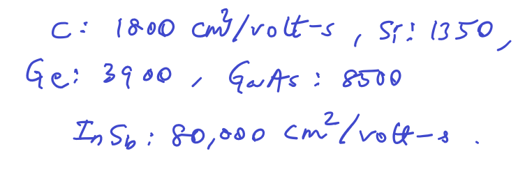

For electrons (strongly n-type semiconductors) electrical conductivity is given by, and mobility by: so: . Typically μ ≅ 100 cm²/volt-s.

For strongly p-type semiconductors: where P is hole concentration and with hole mobility μ_h hole conductivity σ_h is given by: σ_h=Peμ_h.

We see that conductivity is directly proportional to mobility. If both donor and acceptor impurities are present in a semiconductor we can write: . i.e. total conductivity is due to conductivity of both electrons and holes, its the same statement for mobility as well.