Electric Dipole: Potential And Electric Field Due To Dipole, Lecture-9.

Lectures on Electricity and Magnetism — new series of lectures – EML – 9.

All articles in this series will be found here. Click on link to left or search for menu “E AND M BASICS” on top.

Electric Dipole: Dipole Moment, Potential, Electric Field Force And Torque, Lecture-9

Electric Dipole

An electric dipole is a system of two equal and oppositely signed charges +q and -q separated by a distance d. Atomic phenomena can often be modelled in terms of dipoles, so its important to study the dipole in detail.

If we choose the origin at mid point of the dipole then the positive charge +q lies at $\frac{\vec{d}}{2}$ and the negative charge -q lies at $-\frac{\vec{d}}{2}$ . This is shown in the following diagram.

**Diagram 1**: An electric dipole: a system of 2 equal and oppositely signed charge. We would like to determine electrostatic potential and electrostatic field at a point referenced by position vector r.

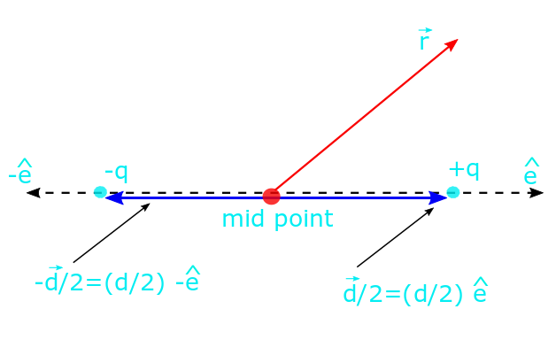
We define the electric dipole moment vector μ or p as a vector with the magnitude of product of charge of one pole (q here) into the distance between the poles (d here), whose direction is given by a unit vector running from the negative pole towards the positive pole. Thus the magnitude of the dipole moment in our example here is p = μ = qd and its direction is ê i.e. p = μ = qdê.

+ click to see more about this article

This article belongs to a group of lectures I intend to prepare for their online dissemination — these were delivered in a physical format, beginning with hand written notes that were delivered in a classroom full of students. This series is on Electricity and Magnetism and bears the name sake Electricity and Magnetism Lectures and the number of the lecture will be appended to the end to reflect the same. eg the current lecture will be named EML – 9 . This lecture was delivered to honors students on 15th Feb 2017.

In the meanwhile if you can’t wait and you need some of these concepts at the earliest, here is a slide-share presentation I had made roughly 5 years ago that consists of “some of the things” an undergrad needs: Electricity and Magnetism slides. There are other slides on different topics at that account of mine on slideshare.net (such as; Introduction to Quantum Mechanics , and these are quite well received by the community for their usefulness).

Electrostatic Potential Of A Dipole

The electrostatic potential for such an arrangement (i.e. a dipole) can easily be written; 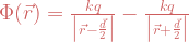$\Phi(\vec{r})=\frac{kq}{\big| \vec{r}-\frac{\vec{d}}{2} \big|} - \frac{kq}{\big| \vec{r} + \frac{\vec{d}}{2} \big|}$ . Its based on the expression for potential of a single charge and superposition principle. You can see the explanation how this is derived in the following show/hide box.

+ Click if you wanna see the explanation how this is done.

We defined the electrostatic potential in lecture EML-4, as the work done against the Coulomb electrostatic force experienced by a test charge (of unit magnitude and positive sign) from infinite distance to a given reference point r. In the scenario that no charge distributions are present at infinite dimensions we obtain an expression for the potential of a single charge Q (that produces the field and the potential in the first place). This potential Φ(r) is given as $\Phi(r)=\frac{W(\infty \to r)}{q}=kqQ \Big[ \frac{1}{\infty}-\frac{1}{r}\Big]\times\frac{1}{q}=\frac{kQ}{r}$ . We then replaced Q by q, where we understand that q is no more the test charge (reference charge) but the source charge that produces the field and the potential.

We also mentioned the superposition principle where if two source charges (of equal magnitude q) are present in their respective locations, their potential would be simply the sum of the potential due to the individual source charges. Since the charges are no more present at origin we need to take the relative vector called separation vector as the distance at which we are calculating field and potential (this vector is usually expressed with the curly r symbol, but we are technically not equipped to do so here). For one charge, the -ve one the separation vector is: $\vec{r}+\frac{\vec{d}}{2}$ and for the other the positive the separation vector is: $\vec{r}-\frac{\vec{d}}{2}$ . See Diagram 1 above for this assertion.

The vector r makes an angle of θ with the vector d (see Diagram 1 above) so we can use the simple results of vector algebra called cosine law (see diagram and expression below), and write; $\Phi(\vec{r})=\frac{kq}{\big( r^2+\frac{d^2}{4}-rd\cos\theta \big)^{\frac{1}{2}}} - \frac{kq}{\big( r^2+\frac{d^2}{4}+rd\cos\theta \big)^{\frac{1}{2}}}$ . The cosine law gives magnitude of a resultant vector from its components, by using the dot product of the resultant vector with itself as the square of its magnitude.

+ Click to see more about the cosine law.

Cosine law gives magnitude of a resultant vector from its components, by using the dot product of the resultant vector with itself as the square of its magnitude.

Cosine Law: $R=\sqrt{A^2 + B^2+2AB\cos\theta}\,\,\,for\,\,\, \vec{R}=\vec{A}+\vec{B}$ . Sine Law: The angle made by resultant vector R with component vector A is given by: $\sin\alpha=\frac{B}{R}\sin\theta$ and $\tan\alpha=\frac{B}{A+B\cos\theta}\sin\theta$

In the limit d << r (i.e. $\frac{d^2}{r^2}<< 1$ ) we can use the binomial expression, after retaining only first order term (d/r). $\big( r^2+\frac{d^2}{4}\pm rd\cos\theta \big)^{\frac{1}{2}}\approx r\big( 1\pm \frac{d}{2r}\cos\theta \big)$ . Now the potential due to the dipole takes the form: $\Phi(\vec{r})=\frac{kq}{r\big(1-\frac{d}{2r}\cos\theta\big)} - \frac{kq}{r\big(1+\frac{d}{2r}\cos\theta\big)}\simeq \frac{kqd}{r^2}\cos \theta$ . Now we can use the definition of electric dipole moment that we mentioned above, with θ the angle between the reference vector r (from the mid point as shown in Diagram 1 above) and the dipole vector p: $\boxed{\Phi(\vec{r}) = k\frac{\vec{p}\cdot \vec{r}}{r^3}=\frac{1}{4\pi \epsilon_0}\frac{\vec{p}\cdot \hat{r}}{r^2}=\frac{1}{4\pi \epsilon_0}\frac{p \cos \theta}{r^2}}$ .

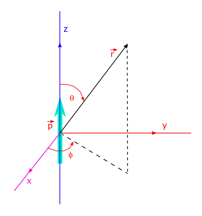
Lets redraw a more fullscape diagram to show the situation. The following diagram shows the spherical polar coordinate system of r, θ and φ juxtaposed on the Cartesian coordinate system of x, y, z for any vector r. The dipole moment vector p is aligned along the positive z-axis making an angle θ with the reference vector r.

The dipole moment vector p is aligned along the positive z-axis making an angle θ with the reference vector r in the spherical polar coordinate system of r, θ and φ juxtaposed on the Cartesian coordinate system of x, y, z for any vector r.

Electrostatic or Electric Field Of An Electric Dipole

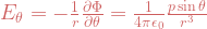
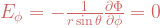
From the given expression above for the electrostatic potential of an electric dipole moment we can calculate the electrostatic or electric field created by the dipole. As you can see in the diagram above, we have taken the z-axis to be the direction of the dipole moment vector p. The electric field is the negative potential gradient given by the expression, $\vec{E}=-\vec{\nabla}\Phi$ which we have discussed in detail here.

Electric Field Due To Electric Dipole In Spherical Coordinate System

The gradient operator ( a vector operator) which appears on the right hand side (and acts on scalar as well as vector fields, albeit in different ways, but here on the scalar field Φ) is given as: 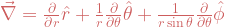$\vec{\nabla} = \frac{\partial }{\partial r} \hat{r} + \frac{1}{r}\frac{\partial }{\partial \theta} \hat{\theta}+\frac{1}{r\sin \theta}\frac{\partial }{\partial \theta} \hat{\phi}$ , in spherical polar coordinate system. Accordingly we can find the electric field component wise.

The radial component is 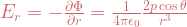$E_r = -\frac{\partial \Phi}{\partial r} =\frac{1}{4\pi \epsilon_0}\frac{2p\cos \theta}{r^3}$ , the polar angle component is $E_{\theta}= -\frac{1}{r}\frac{\partial \Phi}{\partial \theta} =\frac{1}{4\pi \epsilon_0}\frac{p\sin \theta}{r^3}$ and the azimuthal component is $E_{\phi}= -\frac{1}{r\sin\theta}\frac{\partial \Phi}{\partial \phi} =0$ . The resultant electric field then due to the dipole oriented along the z-axis (θ = 0) $\vec{E}_{dipole}(r,\,\theta) = \frac{1}{4\pi \epsilon_0}\frac{p}{r^3} (2\cos\theta\,\, \hat{r}+\sin\theta\,\, \hat{\theta})$ . This is a coordinate dependent form. i.e. its useful only where the spherical polar coordinate system is purported to be implemented.

Electric Field Due To Electric Dipole In Coordinate Independent Form

We can cast this expression into its coordinate independent form so that its useful in any arbitrary coordinate system for vector analysis. For that we first off all need the following transformation rules (for unit vectors) in Spherical Polar Coordinate and Rectangular Cartesian Coordinate system.

Note, unit vector transformation rules between Spherical polar and Cartesian system: 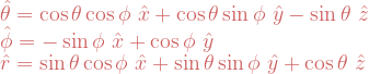$\hat{\theta} = \cos\theta \cos\phi \,\,\hat{x} + \cos\theta \sin\phi \,\,\hat{y} - \sin\theta \,\,\hat{z}\\ \hat{\phi} = -\sin\phi \,\,\hat{x} + \cos\phi \,\,\hat{y}\\ \hat{r} = \sin\theta \cos\phi \,\,\hat{x} + \sin\theta \sin\phi \,\,\hat{y} + \cos\theta \,\,\hat{z}$ . Also $\hat{\theta}\cdot\hat{z}=-\sin\theta=\cos (\pi/2+\theta)$ so angle between $\hat{\theta}$ and $\hat{z}$ is (π/2)+θ.

θ is the angle between vector $\vec{p}$ and radial unit vector $\hat{r}$ so $\vec{p}\cdot \hat{r}=p\cos\theta$ . But $\hat{\theta}$ makes angle θ+(π/2) with $\vec{p}$ (i.e. $\hat{z}$ ) as we mentioned in the note above. So, $\vec{p}\cdot \hat{\theta}=p\cos(\pi/2 + \theta)=-p\sin\theta$ , this leads to: $\vec{p}=(\vec{p}\cdot \hat{r})\hat{r}+(\vec{p}\cdot \hat{\theta})\hat{\theta}=(p\cos\theta) \hat{r}-(p\sin\theta)\hat{\theta}$ .

So the spherical coordinate form of the dipole electric field now becomes: $\vec{E}(r,\,\theta) = \frac{1}{4\pi \epsilon_0}\frac{1}{r^3} (2\cos\theta \,\,\hat{r}+\sin\theta\,\, \hat{\theta})=\frac{1}{4\pi \epsilon_0}\frac{p}{r^3} (2(\vec{p}\cdot \hat{r})-\vec{p}+(\vec{p}\cdot \hat{r}) \,\,\hat{r}$ . This leads to the final expression for the coordinate independent form of the electric field of the electric dipole moment: $\boxed{\vec{E}_{dipole}(r,\,\theta) =\frac{1}{4\pi \epsilon_0 r^3} \big[(3(\vec{p}\cdot \hat{r})-\vec{p}\big]}$ .

Force, Torque And Potential Energy On An Electric Dipole In A Uniform Field

The net force on an electric dipole present in a uniform electric field is zero as forces act in opposite directions for oppositely signed charges. (The electric field must be uniform for this assertion). But there is a net amount of torque: $\vec{N} = \vec{p}\times \vec{E}$ , which does not vanish in a uniform electric field. The torque N is calculated as follows.

Calculating torque on an electric dipole in a uniform electric field: $\vec{N}= \vec{r}_{+}\times \vec{F}_{+} + \vec{r}_{-}\times \vec{F}_{-}\\=\frac{1}{2}\vec{d}\times (q\vec{E})+[-\frac{1}{2}\vec{d}\times (-q\vec{E})]\\=\frac{1}{2}q\vec{d}\times\vec{E}+\frac{1}{2}q\vec{d}\times\vec{E}\\=\frac{1}{2}\vec{p}\times\vec{E}+\frac{1}{2}\vec{p}\times\vec{E} \\= \vec{p}\times\vec{E}$ .

It can also be shown that the potential energy of an electric dipole in a uniform electric field is given by $U=-\vec{p}\cdot\vec{E}$ . We will add some content here if time permits in the near future.

Rate this:

Comments

2 responses to “Electric Dipole: Potential And Electric Field Due To Dipole, Lecture-9.”

Electrostatic Potential Energy Of Different Charge Configurations. Lecture-10, 11. – M Dash Foundation: C Cube Learning

July 10, 2020

[…] potential energy and electrostatic potential for simple electrostatic charge distributions here and here. In this lecture we will take it up a notch and discuss advanced cases and evaluate their […]

LikeLike

Conductors in Electrostatic Field – M Dash Foundation: C Cube Learning

July 21, 2020

[…] some of the electric field, applied externally. You can learn the basics of electric dipole moments here in lecture […]

LikeLike