Uniqueness Theorem in Electrostatics, Lecture 12.

Lectures on Electricity and Magnetism — new series of lectures – EML – 12.

All articles in this series will be found here. Click on link to left or search for menu “E AND M BASICS” on top.

Uniqueness Theorem In Electrostatics

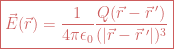
An electric field for a point charge is obtained from the Coulomb’s inverse square law, the electrostatic fields are introduced in lecture EML-1 in much detail. We saw there that this field is given by the following expression: $\vec{E}(\vec{r}) = \frac{1}{4\pi \epsilon_0}\frac{Q \vec{r}}{r^3}$ if the source charge producing the field is at the origin and the reference point for the calculation of the field is at the position vector: r. If instead we are adamant in leaving the source charge at any arbitrary position given by vector r’ and want to determine the field at a position given by vector r, we slightly modified that expression to: $\boxed{\vec{E}(\vec{r}) = \frac{1}{4\pi \epsilon_0} \frac{Q (\vec{r}-\vec{r}\,')}{(|\vec{r}-\vec{r}\,'|)^3}}$ .

If multiple discrete charges — or a continuous distribution of charge, are present in an arbitrary fashion the superposition principle for the electric field comes into picture. According to this principle, “contribution of each individual element of charge is independent of contribution of all the other elements of charge, hence the total contribution is the sum total of contribution of each individual element“, accordingly for a continuous distribution of charge: $\boxed{\vec{E}(\vec{r}) = \frac{1}{4\pi \epsilon_0} \int d^3r\,' \frac{\rho(\vec{r}\,') (\vec{r}-\vec{r}\,')}{(|\vec{r}-\vec{r}\,'|)^3}}$ . Here ρ is the volumetric charge distribution.

We already know that the electrostatic field is the negative potential gradient and inversely the electrostatic potential is the negative line integral of the electrostatic field. We discussed this in much detail, here, in EML-4. The electrostatic potential is thus given as: $\boxed{\Phi(\vec{r}) = - \int_{\infty}^{\vec{r}} \vec{E}(\vec{r}\,')\cdot d\vec{r}\,'}$ . Also we can solve for the electrostatic potential Φ from the Laplace equation (∇ ²Φ = 0) or Poisson equation (∇²Φ = -ρ/ε₀) and from there find the electrostatic field E. The Laplace and Poisson equations are discussed in much detail (with derivation, applications and problems) here in EML-5, 6, 7 and 8.

ρ is not always known a priori. But we can solve electrostatics problems for the electrostatic potential Φ and for the electrostatic field vector E, using the Laplace and Poisson equation, when partial information about these variables (potential Φ and field E) are available.

Boundary Value Conditions

The partial knowledge of the value of the electrostatic potential Φ or its normal derivative (i.e. vector E, which is the electrostatic field) on a specified number of surfaces (S₁, S₂, … etc) is known as the Boundary Value Conditions. The electrostatic problems become a method to solve a differential equation with given boundary values.

Accordingly there are two types of boundary value conditions.

Dirichlet Boundary Value Conditions: when the electrostatic potentials are known on the surfaces this is known as Dirichlet Boundary Value Condition: E.g. Φ(S₁) = V₁, Φ(S₂) = V₂ etc. The solutions to Laplace or Poisson equations must satisfy these boundary value conditions.
Neumann Boundary Value Conditions: when the normal derivatives of the electrostatic potential Phi are known on the surfaces this is known as Neumann Boundary Value Condition: E.g. E(S₁), E(S₂) etc are known. The solutions to Laplace or Poisson equations must satisfy these boundary value conditions.

Linear Combination Of Solutions

Let V₁, V₂, V₃, …, V_n be the values of the electrostatic potential that are specified on the surfaces of the conductors, viz. S₁, S₂, …, S_n. If Φ₁, Φ₂, … etc are solutions that satisfy the Laplace or Poisson equation and in addition satisfy the given boundary value conditions, then: Φ = a₁Φ₁ + a₂Φ₂ + a₃Φ₃ + … + a_nΦ_n is also a solution to the Laplace or Poisson equation that satisfies the boundary value conditions specified in the problem because Laplace and Poisson equations are linear differential equations. Mathematically: ∇²Φ = a₁∇²Φ₁ + a₂∇²Φ₂+ … + a_n∇²Φ_n= 0.

Uniqueness Theorem

Statement Of Uniqueness Theorem

The uniqueness theorem can be stated as the following: “To every boundary value condition there exists a unique solution to the Laplace equation. Two solutions of Laplace equation that satisfy the same boundary value condition are (i) same for Dirichlet Boundary Value Condition and (ii) differ by an additive constant for Neumann Boundary Value Condition.

Proof Of Uniqueness Theorem

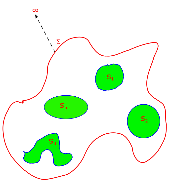
Lets consider the following simplistic diagram to describe the required volumes and boundaries in the proof of the uniqueness theorem.

A system of conductors with surfaces, S1, S2, ..., Sn and a closed surface Σ which encloses the region R — A system of conductors with surfaces, S₁, S₂, …, S_n and a closed surface Σ which encloses the region R.

Lets consider a system of conductors with surfaces, S₁, S₂, …, S_n and a closed surface Σ which encloses the region R, excluded by the surfaces of the conductors, that we just mentioned.

There is no charge in region R hence Laplace equation (∇ ²Φ = 0) is valid. Lets say Φ₁ and Φ₂ are two solutions to the Laplace equation so that they satisfy the same boundary conditions on the surfaces: S₁, S₂, …, S_n. Lets consider: Φ = Φ₁ – Φ₂. Φ is a solution to the Laplace equation since: ∇ ²Φ = ∇ ²Φ₁ – ∇ ²Φ₂ =0, as Φ₁ and Φ₂ individually satisfy Laplace equation.

Lets find the divergence of $\Phi \vec{\nabla} \Phi$ in the volume of region R. We will apply the Gauss Divergence Theorem to the divergence, as explained many times now, this theorem converts the volume integral (left hand side of the equation to be followed) into a surface integral (right hand side), mathematically: $\boxed{\int_V (\vec{\nabla} \cdot \vec{A}) \, d\tau = \oint_S \vec{A}\cdot d\vec{S}}$ — more fittingly the Gauss divergence theorem relates the divergence of the field in the volume bounded by the surface (left hand side) to the flux of a vector field through a closed surface (right hand side). So we have: $\boxed{\int\int\int_R \vec{\nabla} \cdot (\Phi \vec{\nabla} \Phi) \, dV = \int\int_{\Sigma + S_1 +S_2 + ... + S_n} \Phi \vec{\nabla} \Phi \cdot \hat{n}dS}$ . As we have mentioned, S₁, S₂, …, S_n and Σ etc are the bounding surfaces of R.

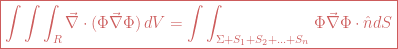
The boundary value conditions could be (i) Dirichlet condition: Φ₁ = Φ₂ or (ii) Neumann condition: $\vec{\nabla} \Phi_1 \cdot \hat{n}=\vec{\nabla} \Phi_2 \cdot \hat{n}$ . This makes the right hand side of the divergence expression (surface integral) zero. We can also take surface Σ such that if Σ → ∞ so that the potentials on this surface are zero (when there are no charges at infinity the potential is set to zero at infinity) and the resulting surface integral is zero.

Thus we get: $\boxed{\int\int\int_R \vec{\nabla} \cdot (\Phi \vec{\nabla} \Phi) \, dV = \int\int\int_R \Phi \nabla^2 \Phi dV + \int \int \int_R (\vec{\nabla}\Phi )^2 dV=0}$ . This we obtained by using the vector identity: $\vec{\nabla}\cdot(\Phi \vec{A})=\Phi\vec{\nabla}\cdot \vec{A}+\vec{A}\cdot \vec{\nabla}\Phi$ . Since Laplace equation is satisfied ∇ ²Φ = 0 in R, the above result means, $(\vec{\nabla} \Phi)^2=0$ , i.e. the gradient of Φ (electric field) is zero. So the value of potential must remain constant in R, and equal to the value specified on the surface.

Now we want to see what this means under Dirichlet condition and under Neumann condition. (i) from Dirichlet condition: Φ₁ = Φ₂ so Φ = 0, and Φ must be zero everywhere in R and that means the two solutions satisfying the same boundary value condition must themselves be same (i.e. unique). (ii) from Neumann condition: $\vec{\nabla} \Phi_1 \cdot \hat{n}=\vec{\nabla} \Phi_2 \cdot \hat{n}$ so $\vec{\nabla} \Phi \cdot \hat{n}=0$ on the surfaces, thus Φ is constant (Φ = Φ₁ – Φ₂ = constant) and so Φ₁ and Φ₂ differ by an additive constant. This proves the assertions we made regarding uniqueness theorem.

+ click to see more about this article

This article belongs to a group of lectures I intend to prepare for their online dissemination — these were delivered in a physical format, beginning with hand written notes that were delivered in a classroom full of students. This series is on Electricity and Magnetism and bears the name sake Electricity and Magnetism Lectures and the number of the lecture will be appended to the end to reflect the same. eg the current lecture will be named EML – 12. This lectures was delivered to honors students on 14th Feb 2017.

In the meanwhile if you can’t wait and you need some of these concepts at the earliest, here is a slide-share presentation I had made roughly 5 years ago that consists of “some of the things” an undergrad needs: Electricity and Magnetism slides. There are other slides on different topics at that account of mine on slideshare.net (such as; Introduction to Quantum Mechanics , and these are quite well received by the community for their usefulness).

Uniqueness Theorem in Electrostatics, Lecture 12.