Phase space, ensemble and Liouville’s theorem

Statistical mechanics lecture — III

“Phase space, ensemble and Liouville’s theorem”

This lecture for the physics honors degree class was delivered on the 8 – January – 2018.

( All “statistical mechanics” series lectures ) Information Go to other available statistical mechanics lectures

You may want to read last two lectures for a better understanding of the present lecture.

Lectures I and II..

( Last two lectures — I and II ) Information Read last two lectures for better understanding

Topics covered in this lecture

a. Ensemble and average — thermodynamic systems

b. Phase space — a classical system

c. Liouville’s theorem — with derivation

Ensemble and average in thermodynamic systems

For a given “macrostate” $(N, \,V, \,E)$ a statistical system, at any instant of time, $t$ , is likely to be found in any one of an extremely large number of distinct “microstates”.

When time passes, the system evolves into different microstates. In due course of time the system exhibits an average behavior of all microstates it passes through.

We can equivalently depict this behavior by envisaging a large number of mental copies of the system, with the same macrostate as the original system, but all the possible microstates, in which the system can exist, all at once. Such a collection of hypothetical or mental copies of the given system is known as an ensemble.

Thus the average behavior of the ensemble is expected to be identical with the time-averaged behavior of the actual physical system. In fact this is one of the fundamental requirements for statistical mechanics to be valid. No matter which mathematical avenue we prefer to meander through we must in the end reach our unique destination of physical validity.

To understand the deeper aspects of this ensemble theory we need to define what is known as “phase space” of a statistical system.

Phase space of a classical system

Let us consider a given physical system with a specified macrostate with $N$ number of particles. There are $3\,N$ position coordinates $q_1, q_2, ..., q_{3N}$ in short $(q_i)$ and $3\,N$ momentum coordinates $p_1, p_2, ..., p_{3N}$ in short $(p_i)$ that characterizes the microstates of the system.

Thus we are in a $6\,N$ dimensional space geometrically. This space so defined embodies the “phase space” of the given physical system represented by $(q_i, \,p_i);\,\,\,\,i = 1, 2, ..., 3N$ . $(q_i, \,p_i)$ is called the “representative point” or the “phase point“.

$q_i$ and $p_i$ are functions of time and satisfy the “canonical equations of motion” given by the following.

$\boxed{\dot{q}_i=\frac{\partial H(q_i, p_i)}{\partial p_i}, \,\,\,\,\dot{p}_i=-\frac{\partial H(q_i, p_i)}{\partial q_i},\,\,\,i=1,2,...,3N}$

$H(q_i, \,p_i)$ is the Hamiltonian of the system.

As time passes by the representative point $(q_i, \,p_i)$ traces a trajectory whose direction is given by: $\vec{v} \equiv (\dot{q}_i, \dot{p}_i)$ .

Due to finite volume $V$ and finite energy $E$ the representative point is restricted to a limited region in phase space.

Note that: $V$ restricts $q_i$ but $E$ restricts both $q_i$ and $p_i$ .

Thus through $H(q_i, \,p_i)=E$ , the trajectory is restricted to a “hyper surface“. If $E \in (E - \frac{1}{2}\Delta , E+ \frac{1}{2}\Delta)$ the trajectory is restricted to a “hyper-shell“.

For an “ensemble theory” the member of the ensemble will keep on changing their microstates, over time. Thus there are a “swarm of representative points” which continually move along respective trajectories of the member in the ensemble.

We now define a “density function” $\rho \,(q,\,p; \,t)$ where $q\equiv q_i$ , $p\equiv p_i$ , $i=1,2,\,...\,,3N$ . Thus $\rho$ gives number of representative points in a given volume of phase space $\big(d^{3N}q \big)\big(d^{3N}p\big)$ , around phase point $(q_i, \,p_i)$ , for all $i$ — i.e. $(q, \,p)$ .

Thus $\rho$ also gives the fashion in which the members of the ensemble are distributed over all possible microstates.

We can take an “ensemble average” of a given physical variable $f (q,\, p)$ as follows.

$\bar{f} = \langle f (q,\, p)\rangle\, = \, \frac{\int f(q, \,p) \rho (q, \,p; \,t) \big( d^{3N}q \big) \, \big( d^{3N}p \big)}{\int \rho (q, \,p;\,t) \big( d^{3N}q \big) \, \big( d^{3N} p \big)}$ .

The integration is carried out over all space in the phase space but has contribution only where $\rho \neq 0$ , i.e. populated regions in the phase space.

An ensemble is said to be stationary if $\rho$ does not depend on time, explicitly: i.e. $\frac{\partial \rho}{\partial t}=0$ , at all times. This would mean ensemble average of a physical variable $f(q, \,p)$ , i.e. $\langle f(q,\,p)\rangle$ is independent of time. Stationary ensembles represent systems in equilibrium.

Liouville’s theorem

Consider an arbitrary “volume” $\omega$ in a relevant region in the phase space, which is bounded by the surface $\sigma$ . Rate of increase of representative points in this volume is given by: $\frac{\partial}{\partial t}\Big(\int\limits_{\omega}\rho \, d\omega\Big), \,\,\,\, d\omega=\big(d^{3N}q\big) \big(d^{3N}p\big)$ .

Flow of phase space points: a surface depicting flow of phase space points across a closed boundary. This leads to an equation of continuity which in turn leads to the Liouville's theorem. — **Flow of phase space points**: a surface depicting flow of phase space points across a closed boundary. This leads to an equation of continuity which in turn leads to the Liouville’s theorem.

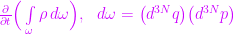
The net rate at which these points would flow out of the volume $\omega$ from the surface $\sigma$ , is given by: $\int \limits_ \sigma \rho \vec{v}.(\hat{n} d\sigma)$ .

By the application of divergence theorem, which converts surface integrals to volume integrals — and vice a versa, the surface integral mentioned above turns into: $\int\limits_\omega div \,(\rho \vec{v})\, d\omega$ .

But divergence is defined in this space by; $div \,(\rho \vec{v})= \sum \limits_{i=1}^{3N} \{\frac{\partial}{\partial q_i} (\rho \dot{q}_i)+ \frac{\partial}{\partial p_i} (\rho \dot{p}_i)\}$ .

Since there are no sources or sinks in the volume, total number of representative points must be conserved. Thus; $\frac{\partial}{\partial t} \int\limits_{\omega}\rho \,d\omega = - \int\limits_{\omega} div \,(\rho \vec{v})\, d\omega$ ;

or by simple algebra, $\int\limits_\omega \{\frac{\partial \rho}{\partial t}\, + div \,(\rho \vec{v})\, \} d\omega=0$ .

This integration is zero identically for all arbitrary volumes 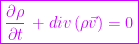$\omega$ . Thus; $\boxed{\frac{\partial \rho}{\partial t}\,+ div \,(\rho \vec{v}) = 0}$ .

The boxed equation is an equation of continuity, for the swarm of representative points depicting the time evolution of the members of the ensemble.

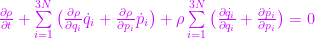
Let us combine the equation of continuity with the definition of the divergence in the phase space.

$\frac{\partial \rho}{\partial t} + \sum \limits_{i=1}^{3N} \big( \frac{\partial \rho}{\partial q_i} \dot{q}_i + \frac{\partial \rho}{\partial p_i} \dot{p}_i \big) + \rho \sum \limits_{i=1}^{3N} \big( \frac{\partial \dot{q}_i }{\partial q_i} + \frac{\partial \dot{p}_i }{\partial p_i} \big) =0$

The $3^{rd}$ term is zero due to equation of motion, which we wrote out at the beginning as a condition that the phase point or representative point was required to satisfy. So if we use the equation of motion to the definition of divergence, coupled with equation of continuity we can see immediately that the $3^{rd}$ term is indeed zero.

$\frac{\partial \dot{q}_i}{\partial q_i} = \frac{\partial ^2 H (q_i, p_i)}{\partial q_i \partial p_i} = \frac{\partial ^2 H (q_i, p_i)}{\partial p_i \partial q_i} =- \frac{\partial \dot{p}_i}{\partial p_i}$

Thus we can write;

$\boxed{ \frac{d\rho}{dt} = \frac{\partial \rho}{\partial t} + [\rho, H] = 0}$ where $[\rho, H]$ is the Poisson bracket.

$[\rho, \,H] \equiv \sum \limits_{i=1}^{3N} \big( \frac{\partial \rho}{\partial q_i} \frac{\partial H}{\partial p_i} - \frac{\partial \rho}{\partial p_i} \frac{\partial H}{\partial q_i} \big)$

The above boxed equation is known as Liouville’s theorem.

It signifies that for an observer moving with a representative point, the “local” density of the representative points stays constant in time. The “swarm of representative points” move in phase space in a manner identical to the motion of an incompressible fluid in physical space.

4 thoughts

Pingback: Lectures on statistical mechanics. Lecture — IV. Microcanonical ensemble. – "Invariance" from M Dash Foundation
Pingback: Maxwell-Boltzmann distribution for a classical ideal gas – M Dash Foundation
Pingback: Test Share Preview – Regina Personal Test Site
Pingback: Concept of movement of the representative points in the phase space ~ Physics ~ ultramadonna.com

M Dash Foundation: C Cube Learning

Invariance: A journal with a difference, where mind meets aspiration

Phase space, ensemble and Liouville’s theorem

Statistical mechanics lecture — III