Waves

Optics Series,  lecture — XII, XIII

These lectures were delivered on 17th and 20th February 2017 ( for 1.5 hours each ) to honors students.

( all optics series lectures ) Go to other available optics lectures

“Waves: traveling waves, differential wave equation, particle and wave velocities”

---

Background: In one of our earlier optics series lecture ( linked below this paragraph ) I had hinted at having waves defined by their pulse shape known as wave profile — or alternatively wave shape or wave form. The wave profile can further be transcribed into forms that represent actual wave motion.

( Earlier lecture: harmonic plane waves ) click to read this article

When the wave profile is laced with the ability to evolve in time, they are called as traveling or progressive waves. The wave shape or wave profile are therefore time-snapshots of the full fledged time varying waves or traveling waves.

Remember that stationary or standing waves are not wave profiles or any snapshots of a single traveling wave. The standing waves are the superposition of an advanced and a retarded wave — that is, one traveling wave moving forward ( also called forward wave ) and another exactly shaped like the forward traveling wave which is moving in the reverse direction ( also called a backward wave ). We studied advanced and retarded waves in the following linked lecture.

( lecture about advanced and retarded waves ) click to read harmonic spherical waves

We have also already dealt with traveling waves in much detail, in two lectures one already linked above (harmonic plane waves ) and another linked below this paragraph. Our present lecture will justify what we have been espousing all along, in those lectures.

Also it is worthwhile to mention that in complex waves that are found in quantum mechanical theories, we have what are called as stationary states, these are like the time-snapshots of the quantum mechanical waves, when these waves are represented through the energy of the system.

Since the full energy or full wave cycle is not necessarily contained in a given amount of time ( the latter is called as a time window ), we have a corresponding uncertainty relation by the name energy – time uncertainty relation.

But when we are talking about an instant of time, stationary states which represent the energy of the ( quantum mechanical ) wave in that instant, are well defined states of energy and also called as eigen – states.

But what would happen if one takes a picture of a dynamic system? There would be fuzzed out region or so called “motion blur” might show up, because these time instants are not well defined eigen states rather they could be superposition of random number of any number of eigenstates.

---

Motion blur: this is outside the scope of this lecture on classical waves and merely linked for the enthusiast, also note that there might be lose ends in that article, which will be reviewed as and when possible.

( Article: motion blur) read an article about any connection between motion blur and relativistic quantum mechanics

---

Travelling waves

Travelling waves: A traveling wave is a self sustaining oscillation of particles of a medium ( also oscillation of any physical quantity without a physical medium ) at different space – time points so that energy is transported across the medium when the oscillation propagates in the medium.

There is no motion of the relevant medium in the ideal description of the wave. The oscillating particles move periodically about their equilibrium locations and in the case of oscillation of physical quantities they take values around their equilibrium values.

The most common examples of waves are mechanical waves: this includes waves on strings, surface waves such as water waves, sound waves, compression waves in solids and liquids.

Depending on the  relation between oscillation direction and wave propagation direction there are two basic types of waves, the longitudinal waves and the transverse waves.

Longitudinal waves

The oscillating particles in the medium move in a direction along the direction of wave motion. Examples of such waves are sound waves and longitudinal wave motion of springs.

Transverse waves

The oscillating particles move in a direction perpendicular to the direction of wave propagation. In case the waves are defined by oscillation of physical quantities ( such as electric field intensity which can exist without a medium ), the oscillation direction is perpendicular to the wave direction. The examples of such waves are electromagnetic waves and transverse waves on strings, eg when the strings of a violin are plucked they produce transverse waves.

Waves move at great speed because there is no associated movement of the medium, there is only advancement of energy.

Let us consider a wave ψ which is moving in + x direction at speed v. So ψ is a function of space coordinate x and time t. Mathematically we write: ψ (x, t) = f (x, t)        —  ( i ).

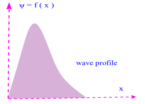
Here f (x, t) represents a particular wave – shape at the instant of time t. Thus wave – profile is the shape of the wave at a given instant of time. Mathematically therefore: ψ (x, t)|_t=0 = f (x, 0) = f(x) ≡ wave profile          — ( ii ).

Waves can take any possible wave forms. Examples of such wave forms are Gaussian ( or bell shape ) and sinusoidal ( or harmonic ) functions.

Gaussian: f(x) = e^-ax2, Harmonic: f(x) = Ae^ikx       — ( iii ).

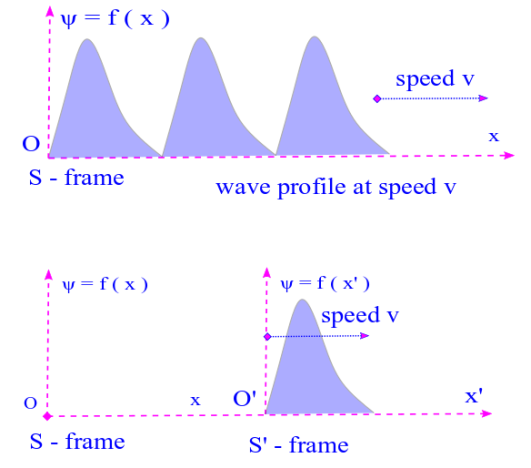
Let us consider waves which do not change shape during propagation. Then the pulse of such waves moves a distance of vt in time t. Consider a particular wave – pulse in the frame of reference S and also in frame of reference S’. The wave pulse moves at speed v in frame S so that in frame S’ it is at rest. Evidently the frame S’ moves at speed v wrt the frame S.

The situation is depicted in the following diagrams. In the frame S’, ψ = f(x’)          — ( iv ). We want to transform ( equation) ( iv ) for coordinates of S. For this we need to recall the Galilean transformation rules or Galilean principle of relativity, according to which: x’ = x – vt          — ( v ), so as a result we have ⇒ ψ ( x, t ) = f ( x – vt )       —  ( vi ).

So ψ ( x, t ) in ( vi ) is a general form of wave function where the wave – disturbance ψ ( x, t ) is moving at speed v in + x direction. ψ ( x, t ) is called a traveling or progressive wave ( in 1 – dimension ) — we can easily change this wave function and any of its related equations to its 3-dimensional form.

We learned that no matter what shape the wave – form has, we can get the corresponding progressive wave by substituting x with x – vt. A harmonic wave – profile gives rise to a harmonic traveling wave and a Gaussian wave – profile that we mentioned a little while ago gives rise to a Gaussian traveling wave.

If a time Δt elapses and the wave pulse has advanced a distance x + v Δt then this implies f [ ( x + v Δt ) – v ( t + Δt ) ] = f ( x – vt ). Thus the wave shape or profile is unchanged. Similarly ψ ( x, t ) = f ( x + vt ) for v > 0 gives a wave moving in the -x direction.

We can easily see the following alternative form to be a valid transformation of the advanced and retarded wave that we just discussed.

Differential wave equation

A differential wave equation is a linear, homogeneous and second order partial differential equation whose solution is the progressive or traveling wave represented by the wave-form: ψ = f ( x’ ). A linear equation is one where two different solutions added together in a linear fashion, is another solution.

i.e. if ψ₁ and ψ₂ are individual solutions to a given differential equation and the linear combination ψ = c₁ ( ψ₁ ) + c₂ ( ψ₂ ) is also a valid solution to the original differential equation then this differential equation is known as a linear differential equation.

This results from the linearity of the terms, that is, each term in the differential equation has a degree either 0 or 1, containing only the functions or constants multiplied by the derivatives and these are grouped in one side and equated to 0.

The square, cubes and the further orders are not allowed for functions or derivatives, but higher order differentiation is allowed. The differential equations would be in-homogeneous if instead of equating the grouped terms to 0 one equates them to another function ( which is not multiplied to any derivative ). This non-zero function is known as a source term ( in all of physics ).

Thus having a constant term ( i.e. a special function ) which is independent of derivatives is the sign of a non-homogeneous or in-homogeneous equation. Equations are called as PDE ( partial differential equation ) if there are more than 1 dependent variables but ODE ( ordinary differential equation ) if there is only one dependent variable.

When a second order differential equation is in the offing, one has two arbitrary constants, since the wave equation is a second order differential equation in this case these constants are represented by the amplitude and the frequency ( or the amplitude and the wavelength ).

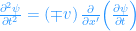
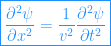
The differential wave equation: We can write: . From the rules of partial differentiation and Galilean relativity that we have used earlier in this lecture:  Similarly: ⇒ . By applying our method once again: and . ⇒ but we have seen already: ⇒ . So finally we have what we call the differential wave equation: .

Harmonic progressive wave

wave parameters and their relations

Lets discuss a wave whose wave – form or wave – profile is given by a harmonic function, that is; a sine or cosine function. Accordingly such waves are called as sinusoidal, harmonic or simple harmonic waves. Its important to study such waves even if they are ideal, because any complicated wave can be considered as a combination of a required number of simple harmonic waves.

The wave profile is given by ψ ( x ) = f ( x ). So  ψ ( x, t )|_{t = 0} = ψ ( x ) = A sin k x = f ( x ), where k is a positive constant known as propagation number or wave number and A is known as the amplitude which gives the maximum possible value of the wave function: ψ ( x ).

Let us create a traveling wave corresponding to the sinusoidal wave profile ψ ( x ). To achieve this we let x through the Galilean transformation. So x → x – vt, where v > 0 and wave moves in the + x direction. So we have: ψ ( x, t ) = A sin k ( x – vt ) = f ( x – vt ).

We have set the differential wave equation in the last section. This harmonic wave – function ψ ( x, t ) = A sin k ( x – vt ) should be a solution to that differential wave equation, namely: .

Take this as a home work and show that this is indeed the case.

Let us define: λ ≡ the spatial period known as wave – length as the distance traversed during which the wave motion changes by ± 2π and the wave – function returns to its original value, before this change. That means when x → x ± λ there is a change in the argument of the harmonic wave function of ± 2π and ψ is unaltered.

So: ψ ( x, t ) = ψ ( x ± λ, t ). Since the traveling wave is based upon a harmonic or sinusoidal variation this implies: sin k ( x – vt ) = sin k [ ( x ± λ ) – vt ] = sin k [ ( x – vt ) ± 2π ] which means kλ = 2π or k = 2π / λ. Similarly when t → t ± τ, ψ is not changed and we have: ψ ( x, t ) = ψ ( x, t ± τ ), τ is called as the time period or temporal period of the wave or wave – function.

Its ( τ ) the time during which one cycle of wave is completed. This gives us a condition in terms of the sine variation. We have: sin k ( x – vt ) = sin k [ x – v ( t ± τ ) ] and sin k ( x – vt ) = sin k [ ( x – v t ) ± 2π ]. From these two we obtain kvτ = 2π or ( 2π / λ ) vτ = 2π or τ = λ / v. But υ = 1 / τ is called as the linear frequency or linear temporal frequency — remember that we can now in analogy with this define the linear spatial frequency.

Always remember by default we do not mention the temporal part, so anytime we must use the analogy privilege in nomenclature we must explicitly specify any spatial variable e.g. by terminology such as spatial frequency and spatial period and so on.

With all the analysis in the section above we see that: v = υ λ, this is the velocity of the wave disturbance and was derived by Newton ( really ). Due to this it is known as Newton’s formula ( for wave velocity ).

Remember that all sorts of waves are always blessed with an amicable relation between their linear frequency and wavelength which multiply to give the velocity. But it is the right time for us to define two other parameters so that we do not commit any mistakes of confusion. We define corresponding parameters and relate them to their linear or angular counterpart as it befits.

Namely; angular ( temporal ) frequency; ω = 2π / τ = 2π υ and  linear wave number or spatial frequency: κ = 1/λ. So there are 4 in total; linear frequency for time, linear frequency for length and their angular counterparts, in the respective order: υ = 1/τ, κ = 1/λ, ω = 2πυ, k = 2πκ.

Let us now state some of the alternative forms for our wave function ψ which can easily be checked by beginning with what we already obtained, namely: ψ ( x, t ) = A sin k ( x ± vt ).

, , ,

Phase velocity

Now we are in a situation where we can define the phase of a wave. We have taken as an example of our wave the harmonic wave – function. Here the total angular argument of the sine or cosine function is called as the phase of the wave. Thus in simple words phase is the angular state — i.e. a function of the space coordinate as well as time coordinate of the wave.

Phase is given by: φ = kx ± ωt when the wave – function is given by: ψ (x, t) = A sin k (x ± vt). If at the initial instant of t = 0 we have x = 0 the wave-function takes the form, ψ (x, t)|_{( t = 0, x = 0 )} = ψ (0, 0) = 0.

But in general: ψ (x, t) = A sin ( kx ± ωt + ε ) where ε is called as the initial phase, phase constant or epoch. Let us evaluate the rate of change of phase with respect to time, at a constant location.

As we can see this gives the angular frequency of the wave: . Similarly the rate of change of phase at a particular instant of time gives us the ( angular ) wave number that we have defined earlier, k, and we have: . According to the rules of partial differentiation: .

So we have: .

This is called as the phase velocity, it is the distance covered by points of constant phase in an unit time. We see that its numerically equal to the wave velocity v and has the same direction as that of the wave velocity if wave is harmonic.

Particle velocity of wave

The particle motion in a medium is described by a velocity which is different from the wave or phase velocity.

, then; .

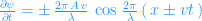
Thus maximum particle velocity is given by: .

Group velocity

There is yet another velocity for waves and its called as group velocity, v_g. When there are multiple waves spanning a region spatially or temporally, the phase of different υ or λ move at different phase velocity. Overall we have v_g = ∂ω/∂k instead of v_p = ω/k.