Matrix formulation in geometrical optics

Optics series, lecture — V

This is the 5th lecture for the physics honors class, delivered on 3rd February 2017.

( All Optics series lectures ) Read other available lectures in optics series

“Matrix formulation in geometrical optics”

In this lecture we will learn about

a. Translation matrix

b. Refraction matrix

c. System matrix

In this lecture, we will discuss about one of the most interesting and powerful methods in geometrical optics. As we have discussed in lecture — III, geometrical optics is that segment of optics in which we are limited to a situation when the wavelength of light is negligible, eg $\lambda$ is insignificant compared to the size of the objects that the light wave interacts with.

We will learn a great deal of detail about what exactly the light wave is, in the future lectures of this series. Many of these are already available in this website, e.g. see the second link below.

( lecture — III ) Read to know more about “geometric optics”

( Waves ) Read about light as wave

As a consequence light ( waves ) can be considered as rays or geometrical straight lines and the nuances of light as wave undulations can be postponed to a happy hour.

Ray tracing

In the geometric optics limit any general optical system can be associated with a ray which can be traced through two basic types of traversal of the ray: translation and refraction. The law of refraction is therefore the central tool for ray-tracing. A ray can be described in an optical system by its coordinates. We will soon define the ray coordinates.

Our goal is to find the matrix which governs the displacement of the ray from one coordinate to another coordinate, as the ray travels from one geometric point to another. This will enable us to study simple as well as much more complicated systems in the most effective and powerful way as we will see.

Lets discuss the basic matrices available for ray tracing when the ray travels from one coordinate to another in the following two cases.

I. Translation matrix: translation matrix is relevant when light travels in a straight line motion in a homogeneous medium
II. Refraction matrix: refraction matrix is relevant for refraction occurring at the interface of two different media

In general therefore the net traversals of the ray can constitute of any number of translations and any number of refraction. A reflection would merely be two translations and a general refraction can be construed from a refraction as well as a translation as we will see.

A most generalized optical system can therefore have $n$ numbers of translations and $s$ numbers of refraction matrices so to say, in their respective orders. The total or resultant matrix would be called a system matrix.

I. Translation matrix

Lets us consider a ray that traverses an optical medium in a straight line, at any angle. This is called as a translation, as the only change the ray undergoes is a translation or straight-line shifting of coordinates. Needless to say this enforces us to realize the ray is limited to a single homogeneous medium.

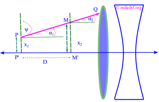
Matrix formulation in geometrical optics: Translation refers to ray tracing in a single homogeneous medium. Ray coordinates are transformed from one point to another through a powerful matrix formulation of optical systems. Photo Credit: mdashf.org — **Matrix formulation in geometrical optics**: Translation refers to ray tracing in a single homogeneous medium. Ray coordinates are transformed from one point ( eg P ) to another point ( eg M or Q ) through matrix formulation of the optical system. **Photo Credit**: mdashf.org

Note that in the above diagram we have shown two different lenses, translation matrix will help us only as far as point Q. We will need further formulation ( refraction matrix ) to be able to see whats going to happen inside of one or more than one lens or any other kind of optical media.

The ray would be completely characterized if we could specify the required number of coordinates of the ray, howsoever complicated it is. In our case it is simple, a straight-line. Therefore we need to specify coordinates of any two points to completely specify our ray.

At any one geometric point on the ray, its coordinate is specified by two variables; height $x$ from the axis ( shown in the figure by PP’ for $x_1$ and MM’ for $x_2$ ) and angle from the axis by $\psi$ or $\alpha$ ( eg $\alpha_1$ or $\alpha_2$ ).

We defined our ray at two points — hence defined it completely, by specifying two coordinates ( height and angle are the coordinates of the ray ) — at two different geometric points ( P and M are the geometric points of the ray ): i.e. by the coordinates ( of the ray ) $(x_1, \alpha_1)$ at geometric point P and by the coordinates ( of the ray ) $(x_2, \alpha_2)$ at geometric point M.

We define another convenient variable, the optical direction cosine $\lambda$ ; its a step closer towards defining optical paths. The optical direction cosine makes life far easier anytime we are dealing with optical situations. If you are interested to see how optical path is defined follow the link.

( How optical path is defined? ) Click to learn more about optical path

The refractive index $n$ comes in handy even if we enjoy the simplicity in this particular problem of a homogeneous medium. This new variable ( optical direction cosine ) is given by $\lambda = n \cos \psi = n \sin \alpha$ .

In our figure shown above the ray moves in a straight line in a homogeneous medium hence $\alpha_1 = \alpha_2$ . Also $\boxed{x_2 = x_1 + D \tan \alpha_1 \,\,\,\,eq^n\,\,(1) }$ . If we assume paraxial region this would imply: $\tan \alpha_1 = \alpha_1$ . This would further change the equations that we just had into: $\boxed{x_2 = x_1 + D \alpha_1 \, \,\, \,eq^n\,\,(2) }$ . Also we have from this: $\boxed{\lambda_1 = n_1 \alpha_1 \, \,\, \,eq^n\,\,(3) }$ and $\boxed{\lambda_2 = n_2 \alpha_2 \, \, \, \, eq^n\,\,(4) }$ .

( What is paraxial region? ) click to see what paraxial region means

Again since our medium is homogeneous $n_1 = n_2$ . Since we are moving in a straight line $\alpha_1 = \alpha_2$ so we have: $\boxed{\lambda_2 = \lambda_1 \, \,\, \,eq^n\,\,(5)}$ and $\boxed{ x_2 = x_1 + \frac{D}{n_1}\lambda_1\, \,\, \,eq^n\,\,(6)}$ .

The expressions in $eq^n\,\,(5\,\&\,6)$ can be written in terms of matrices: $\boxed{\begin{pmatrix} \lambda_2\\x_2 \end{pmatrix}= \begin{pmatrix} 1&0\\ \frac{D}{n_1} & 1 \end{pmatrix} \begin{pmatrix} \lambda_1\\x_1 \end{pmatrix} \, \,\, \,\, \,\, \,\, \, eq^n\,\,(7)}$ .

Thus a ray at coordinate $(x_1, \alpha_1)$ goes to coordinate $(x_2, \alpha_2)$ and this motion is represented by a matrix known as the translation matrix $T$ where, $\boxed{T=\begin{pmatrix} 1 & 0 \\ \frac{D}{n_1} & 1 \end{pmatrix} \, \,\, \,\, \, det(T)=1 }$ .

The actual distance traveled by the ray in the homogeneous medium is approximated by $D$ and this is based on our paraxial assumption. We also see that $det(T)=1$ .

II. Refraction matrix

We determined the form of a matrix that would be responsible to carry a ray from its initial coordinate to its final coordinate if the traversal of the ray under consideration is in a single homogeneous medium and follows a straight line.

A more involved process is that in which the ray gets refracted upon meeting the interface of two media with different refractive indices. By analyzing the traversal of the ray we can determine the matrix that governs the ray traversal for refraction. Accordingly we call it a refraction matrix.

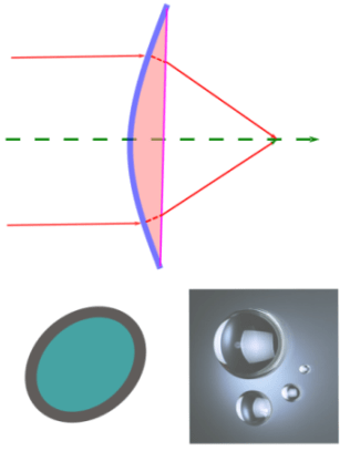
Lets draw a suitable diagram for this situation. We will consider a single refracting surface and leave any further configuration of the surface unaddressed. So we can later extend towards configurations which can have various thickness and different secondary surfaces, after the single surface on left which is spherical with a curvature of radius $R$ .

Matrix formulation in geometrical optics: Refraction refers to ray tracing in inhomogeneous media. Ray coordinates are transformed from one point to another in inhomogeneous media through a powerful matrix formulation of optical systems. Photo Credit: mdashf.org — **Matrix formulation in geometrical optics**: Refraction matrix; refraction matrix refers to ray tracing in inhomogeneous media. Ray coordinates are transformed from one point to another in inhomogeneous media through a powerful matrix formulation of optical systems. **Photo Credit**: mdashf.org

Since the ray now traverses two media while getting refracted at the interfaces of the media we should invoke the Snell’s law in order to constrain the path of the ray.

In addition we are adamant on the paraxial traversal of the ray, that is the ray keeps as close to the optical axis as possible, in height as well as angle, hence sin of angles etc will be approximated to the value of the angles itself, given the angles are already stated in terms of radian consistently.

a. the Snell’s law is given by $\boxed{n_1 \sin \theta_1 = n_2 \sin \theta_2\,\,\,\,\,\,\,\, eq^n\,\,(8)}$ and b. the paraxial assumption is given by $\boxed{n_1 \theta_1 = n_2 \theta_2 \,\,\,\,\,\,\,\, eq^n\,\,(9)}$ .

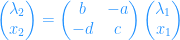
Also we write the relations between angles as shown in the above diagram so that we can express everything in terms of our previously defined ray coordinates, in terms of $(\lambda, \alpha)$ .

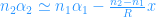
So we have $\boxed{\theta_1 = \phi_1 +\alpha_1 ,\, \,\,\, \theta_2 = \phi_1 + \alpha_2 \,\,\,\,\,\,\,\, eq^n\,\,(10)}$ where $(\alpha_1 \,\,\&\,\, \alpha_2)$ are angles made by the incident ray and the refracted ray with the z-axis, that is, the optical axis. Also $\phi_1$ is the angle made by the normal ( shown as N ) to the refracting spherical surface, with the z-axis.

$(n_1\,\,\&\,\,n_2)$ are the refractive indices of the medium prior to the refracting surface and the medium following the refracting surface respectively.

Our paraxial assumption means 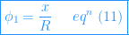$\boxed{\phi_1 = \frac{x}{R}\,\,\,\,\,\,\,\, eq^n\,\,(11)}$ . Thus we have from $eq^n\,\,(9) \,\,\&\,\, eq^n\,\,(10)$ , $n_ 1(\phi_1 + \alpha_1) = n_2(\phi_1+\alpha_2)$ and using $eq^n\,\,(11)$ we have: $n_2 \alpha_2 \simeq n_1\alpha_1 - \frac{n_2 - n_1}{R}x$ .

If we define $P= \frac{n_2 - n_1}{R}$ we would have $\boxed{\lambda_2 = \lambda_1 - Px \,\,\,\,\,\,\,\, eq^n\,\,(12)}$ . $P$ is known as the power of the refracting surface.

Now we note that the height of the ray at point-P before and after the refraction is the same so: 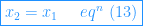$\boxed{x_2 = x_1\,\,\,\,\,\,\,\, eq^n\,\,(13)}$ . $eq^n\,\,(12) \,\,\&\,\, eq^n\,\,(13)$ can together be written as a matrix equation: $\boxed{\begin{pmatrix} \lambda_2 \\ x_2\end{pmatrix}= \begin{pmatrix} 1 & -P \\ 0 & 1\end{pmatrix} \begin{pmatrix} \lambda_1 \\ x_1\end{pmatrix}}$ . $\boxed{R=\begin{pmatrix} 1 & -P \\ 0 & 1\end{pmatrix}}$ is called as the refraction matrix so that $det(R) = 1$ .

III. System matrix

In general any optical system is made-up of a series of refracting and translating motions of a ray. We can thus write a general matrix which transforms the coordinates from one point of the configuration to another, under our paraxial assumption.

$\begin{pmatrix} \lambda_2 \\ x_2 \end{pmatrix} =\begin{pmatrix} b & -a \\ -d & c\end{pmatrix}\begin{pmatrix} \lambda_1 \\ x_1 \end{pmatrix}$ where $S =\begin{pmatrix} b & -a \\ -d & c\end{pmatrix}$ is called as the system matrix. Accordingly a system matrix is a product of any number of possible refraction and translation matrices. Its easy to see that $det(S) = 1$ as well since $det(R) = 1$ , $det(T) = 1$ and $S = RT$ .

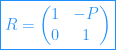
This implies that the elements of the system matrix in general satisfy the condition $bc - ad= 1$ . $(b\,\,\&\,\,c)$ are dimensionless, $a$ has the dimension of inverse length and $d$ has dimension of length.

The matrix in this form is also called the ABCD matrix owing to the symbols of the elements, $a, b, c, d$ .

One thought

Pingback: Application of matrix method to thick lens. « Invariance Publishing House

M Dash Foundation: C Cube Learning

Invariance: A journal with a difference, where mind meets aspiration

Matrix formulation in geometrical optics