Thevenin’s and Norton’s theorem. Complimentary lecture.
Analog systems and applications — complimentary lecture.
This article belongs to a series of lectures on analog electronics, the paper goes by the name “Analog Systems and Applications” for the physics honors degree class. All lectures of this series will be found here. This lecture is intended to be complimentary in nature. It wasn’t delivered to any class of students; but its of much interest and usefulness that it is intended to prepare towards better understanding of the course and outside if the need arises. The offline version was prepared on 29th July 2017.
Today we will discuss the idea of current and voltage sources and the related Norton’s and Thevenin’s theorems. These are immensely useful in understanding many electrical circuits. The content was understood from the “electronic principles, 7th edition” by Albert Malvino and David J Bates, a text which I also followed in developing some of the preliminary materials about semiconductors in this series, in delivering those lectures to the honors students (of 4th semester BSc degree).
Voltage sources.
An ideal DC voltage source produces a constant voltage across the load resistor. Eg a perfect battery (which incidentally doesn’t exist in the real world, its like a spherical cow) is one with zero internal resistance. If an ideal voltage source (say of 10 volt) is connected to a variable load resistor (its not same as varistor, which are resistance that depend on applied voltage) — of resistance say 1 Ω to 10 MΩ then the voltmeter connected across the load will read 10 volt, exactly same as voltage supplied by the source. The current across load resistor would change only if the resistance across it alters.
Now lets see what happens in the real world? (The real world is especially dreadful in love relationships ain’t it? Thankfully we got a good hold on electronic circuits.) Its something where we apply something called a second approximation. The first approximation is where we considered the source to be ideal, i.e. we assumed the source resistance to be zero. In the second approximation though we impart some real practical value to the source resistor and place it in series with the voltage source. The potential drop across this source resistance now decreases the value of the potential drop across the load resistance, from its ideal value (of say 10 volt that we assumed earlier).
The value of voltage across the load resistor can come closer to its ideal value at the voltage source when we increase the load resistance to a value far greater than the source resistance. At 100 times more than source resistance the load resistance produces a voltage within 1% of its ideal value. I.e. when load resistance is more than 100 times the resistance of the source, the load voltage keeps within 99-100% of the ideal source voltage value. The region greater than such a load resistance value is known as stiff region as here the ideal source voltage value is seen across the load, within a stipulated error of 1 or less than 1 %.
This is depicted by the following diagram.
The voltage source and stiff region. The stiff region is 99% accurate when load resistance is 100 times larger than the source resistance.
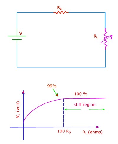
In a stiff voltage source RS < 0.01 RL, RS = 0.01 RL or RL(min) = 100 RS. This definition for stiff voltage source is valid for AC as well as DC sources. But the second approximation (source resistance) is valid for AC only at low frequencies. For higher frequencies we need to consider lead inductance and stray capacitance as well.
Current sources.
Now let us discuss the current sources. A DC current source produces a constant load current at various values of load resistances. A battery with a large source resistance is an example of a DC current source. When the load resistance is sufficiently smaller than the source resistance we have a close approximation to an ideal current source. As in the case of voltage source we can take the load resistance to be 100 times smaller than the source resistance to define a stiff region for the current source. This is depicted in the following diagram.
The current source and stiff region. The stiff region is 99% accurate when load resistance is 100 times smaller than the source resistance.
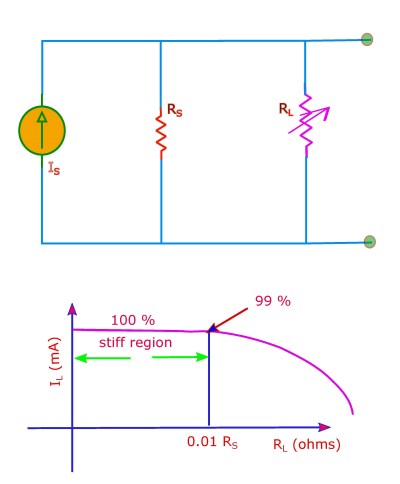
For the current source: 
In a stiff current source RS > 100 RL, RS = 100 RL or RL(min) = 0.01 RS. In a transistor circuit transistors behave as current sources. A transistor acts like a stiff current source and its internal resistance (source resistance) can be neglected.
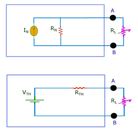
Thevenin’s Theorem.
The Thevenin voltage is defined as the voltage across the load terminals when the load resistor is open (i.e. removed). Its therefore called as open-circuit voltage. Thus Thevenin voltage VTH = VOC. Similarly the Thevenin resistance is defined as the resistance that an ohmmeter measures across the load terminals when all sources are reduced to zero and load resistor is open. Thus Thevenin resistance RTH = ROC. A voltage source is reduced to zero by replacing it by a short (i.e. connecting the open ends after removing the voltage source). But a current source is reduced to zero by replacing it with an open (i.e. leaving the open ends as such after removing the current source).
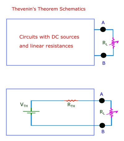
Thevenin’s theorem states that the boxed region in the diagram containing any dc sources and linear resistances is equivalent to the effective circuit where the box is replaced by a voltage source of voltage (VTH) and resistance (RTH) in series with the voltage source.
Thevenin’s theorem is a statement of equivalence between a circuit with dc voltage sources and linear resistances and a simple circuit given by a voltage source of Thevenin voltage value and Thevenin resistance both in series and both determined from the given circuit.
In the equivalent or effective circuit which we can name Thevenin circuit: 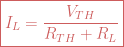
Lets solve a simple example to illustrate how this theorem is implemented in practice.
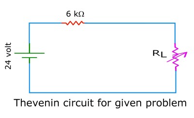
Example problem for Thevenin’s theorem illustration. Diagram 1: given circuit. Diagram 2: determination of Thevenin voltage. Diagram 3: determination of Thevenin resistance.

In diagram 1 above, a circuit is given in terms of DC voltage and linear resistances. In order to find the equivalent Thevenin’s circuit we need to find the Thevenin voltage and Thevenin resistance from this circuit. This we do in diagram 2 and 3 respectively.
In diagram 2 (where the load resistor is open, i.e. removed) there is a current of 8 mA through resistors of 6 kΩ and 3 kΩ. (these are in series with voltage 72 volt.) The 4 kΩ is inconsequential as there is no current through it. The voltage across 3 kΩ is 24 volt and this appears across the terminals A and B. This therefore is the Thevenin voltage value. i.e. VTH = 24 volt.
In diagram 3 the DC source has been replaced by a short (and terminals A and B open). An ohmmeter connected to A and B will see 4 kΩ in series with the parallel combination of 6 kΩ and 3 kΩ.

Thus the Thevenin circuit can be given as in the following diagram.
The equivalent Thevenin diagram to the given problem is determined by calculating the values for Thevenin voltage and Thevenin resistance according to the procedure described above.
Norton’s Theorem.
The Norton current (IN) is defined as the load current when the load resistor is shorted. Thus Norton current is also called short-circuit current. Norton current IN = ISC. Similarly the Norton resistance is defined as the resistance that the ohmmeter would read across the load resistor when all sources are reduced to zero and load resistor is open.
By definition the Thevenin resistance and the Norton resistance are the one and same. Thus RN = ROC = RTH. Just remember that these two resistances Thevenin’s and Norton’s, are placed differently in the circuit, Thevenin’s in series with voltage source and Norton’s in parallel with the current source.
Thus any circuit with DC sources and linear resistances has an equivalent Norton’s circuit given in the diagram below.
The equivalent Norton’s circuit for a circuit with DC sources and linear resistances is determined by calculating the Norton’s voltage and resistance according to steps described above.

Thus Norton’s theorem can be mathematically stated as: 
The Norton’s theorem and Thevenin’s theorem are equivalent formulation and this is based on the Duality principle. According to the duality principle: for any theorem in electrical circuit analysis there is a dual or opposite theorem in which one replaces the original quantities with dual quantities.
Voltage ↔ current. voltage source ↔ current source. series ↔ parallel. series resistance ↔ parallel resistance.
A Thevenin’s circuit and a Norton’s circuit are easily interchangeable according to the following 3 formula: 

Leave a comment