Boundary conditions on electric and magnetic fields.

Electromagnetic theory, lecture — II

This lecture was delivered to the honors class on 22nd December 2017

All electromagnetic theory lectures of this series, will be found here.

“Boundary conditions on Electric and magnetic fields”

Boundary conditions on electric and magnetic field: When electric or magnetic fields go across the boundary of material media their values might or might not change. There are 4 possibilities and we will derive them in this article. These values depend upon the surface current charge densities and the volume charge densities present on the surface of the media. Accordingly the tangential and normal components of electric and magnetic fields have 4 different possibilities. 2 of these change and are named as discontinuous while the other two don’t change and are therefore called as continuous.

boundary bethelsd.org

This image shows two people standing across both sides of a boundary they drew for themselves in the shore of sea. Its a fun way to imagine the values change when someone moves across the boundary, eg the boundary of a nation. When electric or magnetic fields go across the boundary of material media their values might or might not change. There are 4 possibilities and we derive them in this article. — photo-credit; This image shows two people standing across both sides of a boundary they drew for themselves in the sea-shore. Its a fun way to imagine the values change when someone moves across the boundary, eg the boundary of a nation. When electric or magnetic fields go across the boundary of material media their values might or might not change. There are 4 possibilities and we derive them in this article.

Topics covered

A. Summary of Maxwell’s equations — in free space and in material media

B. Integral forms of Maxwell’s equations — by application of vector calculus

C. Derivation of boundary conditions — on electric and magnetic fields

In the last lecture we formulated the Maxwell’s equations, for free space as well as any material medium in their differential form.

Remember that we say free space to mean that the sources of charge densities and sources of current densities that experience our field vectors, viz $\vec{E}$ and $\vec{B}$ — which are produced by other source densities of charges and currents, are non-existent.

That is there is no hindrance or onlookers our $\vec{E}$ and $\vec{B}$ fields meet on their way when they go on a sojourn, in that space. I also hear they call it by the name vacuum. As far as I know I testify, there is no difference between vacuum and free space.

Vacuum simply means for our purpose and many others, there is no glimpse of matter in the space of consideration. It is therefore the simplest of situation to harp on, before we can target our intelligence for achieving more complicated scenario, and yes there certainly are such situations and they take most of our coveted attention in asking us to solve them.

And sooner than later we would be on our toes trying to grasp the burden the more complicated situations would unleash our way. For the time being we focus on free space which means the sources are zero.

Again by sources we mean, not the sources that produce our vector field $\vec{E}$ and $\vec{B}$ but the ones that interact with them, in the path of our fields.

Mathematically free space is: $\rho = 0$ and $\vec{j} = 0$ .

Hence the Maxwell’s equations in matter are given as a set of 4 equations.

i. $\vec{\nabla}\cdot\vec{D} = \rho$

ii. $\vec{\nabla}\cdot\vec{B} = 0$

iii. $\vec{\nabla}\times\vec{E} = -\frac{\partial \vec{B}}{\partial t}$

iv. $\vec{\nabla}\times\vec{H} = \mu_0 \vec{j}+\frac{\partial \vec{D}}{\partial t}$

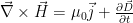
And now its easy to obtain the Maxwell’s equations for free space by setting $\rho = 0$ and $\vec{j} = 0$ .

i. $\vec{\nabla}\cdot\vec{D} = 0$

ii. $\vec{\nabla}\cdot\vec{B} = 0$

iii. $\vec{\nabla}\times\vec{E} = -\frac{\partial \vec{B}}{\partial t}$

iv. $\vec{\nabla}\times\vec{H} = \frac{\partial \vec{D}}{\partial t}$

These 4 equations for free space can also be given in terms of $\vec{E}$ and $\vec{B}$ as:

$\boxed{\vec{\nabla}\cdot\vec{E}=0,\, {\vec{\nabla}\cdot\vec{B}=0,, \vec{\nabla}\times\vec{E} = -\frac{\partial \vec{B}}{\partial t},\,\vec{\nabla}\times\vec{B} =\mu_0 \epsilon_0\frac{\partial \vec{E}}{\partial t}}}$

Differential equations always satisfy boundary conditions for their applicability in physical systems. In order to seek and apply boundary conditions we must first express the Maxwell’s equations into their integral form.

For achieving this we need the magical power of two mathematical theorems. They are known as a. the Divergence theorem and b. the Stoke’s theorem.

a. Divergence theorem: $\int\limits_{\substack{\tau}}(\nabla \cdot \vec {A})\,d\tau = \oint \vec{A}\cdot d \vec{S}$

b. Stoke’s theorem: $\int\limits_{\substack{S}}(\nabla \times \vec {A})\cdot d\vec{S} = \oint \vec{A}\cdot d \vec{l}$

Let $\tau$ be a finite volume in space, $S$ be the closed surface — i.e. the surface bounding the volume, $dS$ be an element of the surface on $S$ and $\hat{n} = \frac{d\vec{S}}{dS}$ be the unit vector normal to the surface at $dS$ , so that it points outward from the enclosed volume.

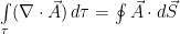
Lets now apply the “divergence theorem” to Maxwell’s equation (i) and (ii).

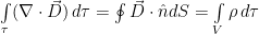
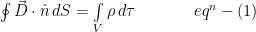
Equation (i) ⇒ $\int\limits_{\substack{\tau}}(\nabla \cdot \vec {D})\,d\tau = \oint \vec{D}\cdot \hat{n} dS= \int\limits_{\substack{V}}\rho \,d\tau$ or, $\oint \vec{D}\cdot \hat{n} \,dS= \int\limits_{\substack{V}}\rho \,d\tau \hspace{42pt}eq^n -(1)$

Equation (ii) ⇒ 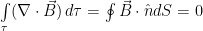$\int\limits_{\substack{\tau}}(\nabla \cdot \vec {B})\,d\tau = \oint \vec{B}\cdot \hat{n}dS =0$ or, $\oint \vec{B}\cdot \hat{n} \,dS= 0 \hspace{42pt}eq^n -(2)$

Let $C$ be a closed contour in space, $S'$ be an open surface which spans the contour, $d\vec{l}$ be a line element on the contour and $dS$ be the surface element on area $S'$ .

Also let $\hat{n}\,'$ be the unit vector normal at $dS$ with direction given according to the right hand rule, applied to the direction of integration along the contour.

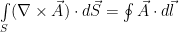
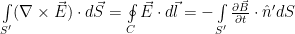
Lets now apply Stoke’s theorem to the remaining two of Maxwell’s equation, in a material medium. Lets apply it to the Ampere-Maxwell equation, i.e. $eq^n\,\, (iv)$ :

$\int\limits_{\substack{S'}}(\nabla \times \vec {H})\cdot d\vec{S} = \oint\limits_{\substack{C}} \vec{H}\cdot d \vec{l} = \int\limits_{\substack{S'}}[ \vec {j} + \frac{\partial \vec{D}}{\partial t}]\cdot \hat{n}'d{S}$ or, $\oint\limits_{\substack{C}} \vec{H}\cdot d \vec{l} = \int\limits_{\substack{S'}}[ \vec {j} + \frac{\partial \vec{D}}{\partial t}]\cdot \hat{n}'d{S} \hspace{42pt} eq^n -(3)$

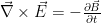
Similarly lets apply Stoke’s theorem to Faraday’s law,

i.e. $eq^n\,\, (iii)$ :

$\int\limits_{\substack{S'}}(\nabla \times \vec {E})\cdot d\vec{S} = \oint\limits_{\substack{C}} \vec{E}\cdot d \vec{l} = - \int\limits_{\substack{S'}} \frac{\partial \vec{B}}{\partial t} \cdot \hat{n}'d{S}$ or, $\oint\limits_{\substack{C}} \vec{E}\cdot d \vec{l} = - \int\limits_{\substack{S'}} \frac{\partial \vec{B}}{\partial t} \cdot \hat{n}'d{S}\hspace{42pt} eq^n -(4)$

Our purpose is to establish relationships between various tangential — i.e. parallel or longitudinal and normal — i.e. transverse or perpendicular components of the $\vec{E}, \vec{B}, \vec{D}$ or $\vec{H}$ fields, that exist across the interface or boundary between two media.

In general these fields are expected to be discontinuous — i.e. differ in their values across the interface, due to presence of surface charge or surface current densities. When they are not discontinuous they are going to be continuous — i.e. bear the same value across the interface.

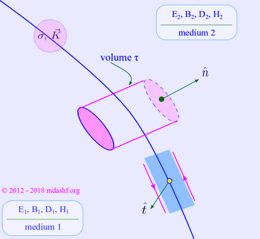
With this in mind let us consider the interface or boundary between two dielectric media characterized by indices 1 and 2. So $E_1, B_1, D_1, H_1$ are the fields in medium 1 and $E_2, B_2, D_2, H_2$ are the fields in the medium 2.

Similarly normal to the interface is denoted by $n$ , ${E^n_1}$ would denote “normal to the interface” component of $E_1$ . Lets also denote tangential component by $t$ . So “on the interface” — same as tangential, component of $E_1$ would be ${E^t_1}$ .

Also let us consider a Gaussian pillbox which straddles the interface. The pillbox is infinitesimal in dimension.

We also consider an infinitesimal contour $C$ whose long arms are on opposite sides of the interface. The normal to the surface enclosed by $C$ would be tangential to the interface.

Boundary conditions on electric and magnetic field: When electric or magnetic fields go across the boundary of material media their values might or might not change. There are 4 possibilities and we derive them in this article. These values depend upon the surface current charge densities and the volume charge densities present on the surface of the media. Accordingly the tangential and normal components of electric and magnetic fields have 4 different possibilities. 2 of these change and are named as discontinuous while the other two don't change and are therefore called as continuous. Photo Credit: mdashf.org — **Boundary conditions on electric and magnetic field**: When electric or magnetic fields go across the boundary of material media their values might or might not change. There are 4 possibilities and we will derive them in this article. These values depend upon the surface current charge densities and the volume charge densities present on the surface of the media. Accordingly the tangential and normal components of electric and magnetic fields have 4 different possibilities. Two of these change and are named as discontinuous while the other two don’t change and are therefore called as continuous. **Photo Credit**: mdashf.org

Lets apply $eq^n \,\,\,1,\, 2$ to the volume of the pillbox in the limit $\tau \to 0$ . In this shallow pillbox the “side” or “curved” surface does not contribute.

Only “top” and “bottom” plane surfaces contribute to the integrals on L.H.S. of $eq^n \,\,\,1,\, 2$ . The top and bottom of the pillbox are parallel and also tangential to the interface.

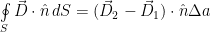
These surfaces have a surface area of $\Delta a$ — say, then: $\oint\limits_{\substack{S}}\vec{D} \cdot \hat{n}\,dS = (\vec{D}_2 - \vec{D}_1)\cdot \hat{n} \Delta a$ and $\oint\limits_{\substack{S}}\vec{B} \cdot \hat{n}\,dS = (\vec{B}_2 - \vec{B}_1)\cdot \hat{n} \Delta a$

R.H.S. ⇒ $\int\limits_{\substack{\tau}}\rho \,d\tau = \sigma \Delta a$

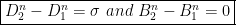
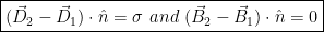
Thus normal components of $\vec{D}$ and $\vec{B}$ on opposite sides of the interface between different dielectric media are given in general as follows.

$\boxed{(\vec{D}_2 - \vec{D}_1)\cdot \hat{n} = \sigma\,\, and \,\, (\vec{B}_2 - \vec{B}_1) \cdot \hat{n}=0}$

same as saying:

$\boxed{D^n_2 - D^n_1 = \sigma \,\, and \,\, B^n_2 - B^n_1 =0}$

For the other two equations, the contour $C$ has short negligible sides crossing the interface and long arms parallel to it — of length $\Delta l$ .

From L.H.S. of $eq^n \,\,\,3,\, 4$ then:

$\oint\limits_{\substack{C}}\vec{E} \cdot d\vec{l} = (\hat{t}\times\hat{n}) \cdot(\vec{E}_2 - \vec{E}_1)\,\Delta l$ and $\oint\limits_{\substack{C}}\vec{H} \cdot d\vec{l} = (\hat{t}\times\hat{n})\cdot(\vec{H}_2 - \vec{H}_1)\,\Delta l$

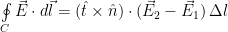
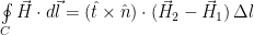
R.H.S. of $eq^n \,\,4$ is zero as $dS =0$ — $area \to 0$ . But right side of $eq^n \,\,3$ does not vanish, if there is a “surface current density” $\vec{K}$ on the interface.

$\int\limits_{\substack{S'}}[ \vec {j} + \frac{\partial \vec{D}}{\partial t}]\cdot \hat{t}d{S}=\vec{K}\cdot\hat{t}\,\Delta l$ — as the 2nd term on the L.H.S. is zero.

Thus tangential components of $\vec{E}$ and $\vec{H}$ are related the following way.

$\hat{n}\times(\vec{E}_2 - \vec{E}_1) = 0 \,\,and \,\, \hat{n}\times (\vec{H}_2 - \vec{H}_1) = \vec{K}$

same as saying:

$\boxed{E^n_2 - E^n_1 = 0 \,\, and \,\, H^n_2 - H^n_1 = K }$

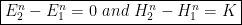
Summary of boundary condition.

As a summary the normal components of $\vec{B}$ and tangential components of $\vec{E}$ are continuous, that is they have the same value. But the normal components of $\vec{D}$ and tangential components of $\vec{H}$ are discontinuous, that is they differ across the boundary, by the surface charge density $\sigma$ and the current density $K=|\vec{K}|$ respectively.

Rate this:

Mahisapat, Dhenkanal, Odisha 759001, India

Comments

3 responses to “Boundary conditions on electric and magnetic fields.”

Electromagnetic Nature of Light — A brief history of light. – "Invariance" from M Dash Foundation

November 1, 2018

[…] I leave this as the most honorable occupation of students: the home-work assignments. The conversion between differential and integral form is achieved here. […]

LikeLike

Helmholtz theorem. Scalar and vector potentials – "Invariance" from M Dash Foundation

November 2, 2018

[…] our previous lectures, lecture – I and lecture — II, we discussed the Maxwell’s equations in free space and in material media. We […]

LikeLike

Laplace And Poisson Equation, Lecture 5, 6, 7 And 8. – M Dash Foundation: C Cube Learning

July 4, 2020

[…] to be imposed on fields when they pass through material media, and we have discussed this here. We will use that result by remembering that normal vector component of the vector D is continuous […]

LikeLike