Electromagnetic Nature of Light — A brief history of light.

---

“Electromagnetic Nature of Light — A brief history of light”

Optics Series Lecture

All optics lectures can be accessed here.

This lecture was delivered on 16th March, yesterday, in a lecture session of 1 and 1/2 hours. This lecture was delivered to physics honors as well as physics elective students.

As I promised in the last lecture, lecture — X,we have our one of the most interesting historical and technical perspective about light, which is also one of my favorite, as I discovered yesterday, or shortly before that, the night before, when I was composing the lecture from scratch.

Let us begin this lecture which has roughly two parts;

1. the history of light and its understanding through the centuries and
2. the electromagnetic nature of light

The second part is intended as the course material for honors as well as elective students but you will be in amusement if you also cover the first part.

A brief history of light

Various optical devices and optical phenomena have been known since close to 4000 years. The optical devices of ancient time includes mirrors, burning glasses, lenses and other magnifying devices.

Accordingly various properties and laws of light were understood and developed since these times. E.g.

a. light was understood to propagate rectilinearly and

b. light was understood to reflect and refract.

There were various laws that were known since these times which catered to the need for explanation of these phenomena.

E.g. reflection was understood to be a phenomena explained by the principle of shortest path — follow link; to know this and other related ideas and their history, in the article: Optical Path.

Laws of refraction were understood either partially or completely, as the centuries or even millennia passed.

Apart from rectilinear propagation of light, it was understood that light moves at infinitely large speed .

Advanced optical devices such as telescopes were developed based on partial and faulty understanding of light which were gradually refined to accommodate better credits of advancement.

Eyes as optical devices, were understood and eye defects could be corrected by using suitable optical devices such as eye-glasses. Albeit all this, light was never understood properly before the 17th CE.

The last 4 centuries saw tremendous leaps of understanding and applications of light. In the 17th CE great progress were made to understand various phenomena exhibited by light such as reflection, refraction and total internal reflection etc.

Descartes proposed light as a longitudinal pressure vibration in elastic medium. Human beings understand by way of imitation and this was the reason light as waves were considered exactly in the image of sound as waves.

The mantra lies in keeping the mind open for successive refinements through acceptance of truth, as ordained eg by experimental facts.

Thus light was considered to be a wave.

During 17th CE, discoveries were made that depicted the diffraction of light. This way light was considered as a rapid vibratory motion of a medium propagating at great speed.

In these similar times Newton had opposing ideas regarding nature of light.

According to Newton light was vibrations of corpuscles or particles with certain emission properties. Despite of this, light was most successfully understood to be a phenomena of wave.

During the same 17th CE Romer performed astronomical experiments on Jupiter’s moon Io and the work of Newton and Huygenss helped ascertain the speed of light to be and respectively.

In the 19th CE wave theory of light received many supporting evidences.

The phenomena of interference and polarization were discovered or understood. Colors of thin films were understood and wavelength of light were determined. The wave theory successfully explained rectilinear propagation of light.

In-fact it was this difficulty about wave theory which kept Newton a staunch supporter of the corpuscular theory of his, rather than the wave theory.

But one by one all hurdles of wave theory of light disappeared at the master strokes of many genius scientists. Similarly the need for explanation for polarization led to the correct view of light as a transverse wave rather than a longitudinal one.

Terrestrial determinations as opposed to astronomical ones as evinced by the work of Romer became order of the day for speed of light.

Fizeu by his toothed wheel method carried out an experiment that established the value of speed of light to a respectable .

Speed of light in water was found to be reduced in comparison to speed of light value in air. This was in conflict with the corpuscular theory of light held in esteem by Newton.

Not many supporters of this view remained any more in the annals of Physics, due also to the demise of the giant that Newton was, to be disproved easily or amicably.

Electromagnetic nature of light

In the 19th CE Maxwell established a relationship between electromagnetic phenomena and light wave, through his experiments and theoretical work. He summarized these relationships in terms of a set of equations known as Maxwell Equations .

I have a short article regarding Maxwell Equations and a highly technical and detailed account of the same in two slide shares presentations, which you might wanna glean over if you have a high appetite for technical matters in physics; article 1, Electromagnetic waves and article 2 Electrodynamics.

Maxwell’s equations evinced the beautiful fact that light waves are nothing but the manifestations of electromagnetic field phenomena which propagate as transverse waves at the speed of light value of c.

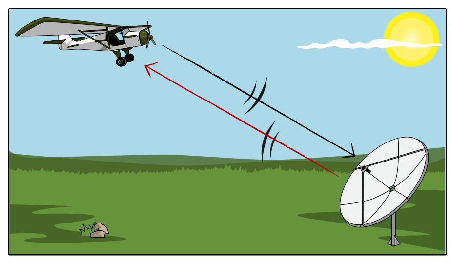
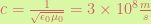
Hertz verified the existence of such waves by his experiments in the same century. Maxwell had shown the most marvelous way to scribe the value of speed of light into the annals of physics: in free space.

But there still were some erroneous understanding of light as a wave. It was incorrectly assumed in the image of previous knowledge that every wave needs a medium to propagate. Hence for light was assigned an all pervasive medium called ether.

This was purported to be a very wispy ubiquitous medium that allows light waves to pass through it without resistance.

Experiments that were performed in the 18th, 19th and 20th centuries could never verify the existence of this luminiferous ether. Finally in 20th CE physicists gave up the idea of this magical but unrealistic medium.

Einstein himself was a brave scientist who supported the invalidity of such a medium in his own work.

For many practical purposes light remains as an electromagnetic wave, to this day, which propagates as a transverse wave in free space at a humongous yet finite and precise invariant speed of 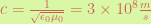 while in other media, it travels at reduced speeds, per the properties of those media.

But there still are many phenomena which can’t be properly explained by such an understanding as a continuous macroscopic wave. For a perfect understanding of light as is possible today, we have to resort to a theory in physics developed in the 1920’s.

This theory is known as Quantum Mechanics.

Let us discuss the electromagnetic nature of light in more detail.

The light as an electromagnetic wave is based on the understanding of electric and magnetic fields.

We know that every static charge produces an electric field given as a vector which exerts a vector force of  on another charge q. So electrostatic charges produce as well as experience electrostatic forces.

Similarly every moving charge produces a magnetic field vector .

This field is the reason any other charge moving at velocity vector , will experience a magneto-static force, given by vector .

Here the sign represents the vector multiplication or the vector cross product — see link to know more, between two vectors namely: and .

Note that in general the moving charges constitute two kinds of current. One is a. steady current and the other b. a non-steady current.

Steady current means a current whose value does not change over time, hence this is the only type of charge motion that produces static magnetic field. D.C. currents are examples of steady currents. The field won’t change its value over time either, as well as the charge in motion that produces it, does not.

So the time derivatives of the current density and the time derivatives of the magnetic field itself, would both be zero in magneto-static conditions.

The other situation of non-steady current — current whose value changes over time, would produce dynamic magnetic fields, that is fields whose value as well, change over time. A.C. currents are examples of non-steady currents. We will read more about the latter type, later.

Like it is in the case of electrostatics, we summarize this by saying: magneto-static — or steady currents produce as well as experience magneto-static forces.

A moving charge creates a magnetic field and a magnetic force, also a moving charge has the qualification to experience such magnetic fields, forces, a static charge would neither create nor experience magnetic force.

This is not all that the unification work of  Maxwell entails.

Every time-varying or time-dependent magnetic field can produce an electric field and thus electric current. On the contrary every time-dependent or time-varying or dynamic* electric field can produce a magnetic field.

*Dynamic; this is the origin of the word dynamics in electrodynamics, as opposed to eg electrostatics.

These two phenomena are together known as electromagnetic induction.

Thus we have a total of 4 phenomena, two time-independent or static and two time-dependent or dynamic effects.

These 4 phenomena are summarized in the form of Maxwell’s equations which can be expressed in both integral and differential forms.

The first two equations of Maxwell’s set of 4 equations are the Gauss law.

The Gauss laws in the case of static electric charge and static electric current, express the fact that the corresponding fluxes are obtained from the bounding surface areas of the given volume, enclosing the respective source charges or source currents.

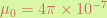
Note that we are concerned only about the free space, where the source charge densities  and the source current densities vector  are null, hence the right hand side is zero, in 1st equation below. To understand the source densities at a deeper and foundational level see this article.

In addition the right hand side of the 2nd equation has to be zero in all cases because there are no magnetic mono-poles.

---

• A. Gauss law — electrostatics: .
• B. Gauss law — magnetostatics: .

The 3rd equation represents the fact that dynamic magnetic field produces electric field — this equation is known as the Faraday’s law of induction.

C. Faraday’s law of induction: .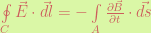

Similarly the 4th equation represents the fact that dynamic electric fields produce magnetic fields. This equation is known as Ampere’s circuital law.

D. Ampere’s circuital law: .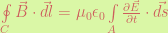

---

Thus the above 4 equations which are called as Maxwell’s equations have been expressed in their integral form and they are applicable to free space.

We can change these into their often useful differential forms, e.g. by using advanced vector theorems: Stokes’ Theorem and Divergence Theorem — or by handy methods of simplifying them in one particular dimension and carrying out any required calculus.

I leave this as the most honorable occupation of students: the home-work assignments. The conversion between differential and integral form is achieved here.

But lets us just write’em down for heaven’s sake. They retain their appellations — i.e. naming for those who are too fidgety with words. Gauss law would still be called Gauss law and so on, irrespective of their integral and differential form.

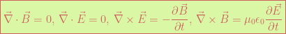
The central idea of an electromagnetic wave is that: an accelerating charge can produce all sorts of electric and magnetic fields.

Thats arbitrary though. In reality the acceleration produces an electromagnetic disturbance, where the E and the B fields are no more independent of each other.

The field directions and the field magnitudes are now interdependent as if someone made them follow the marriage vow: in death do we part.

The vector fields are mutually perpendicular, so that the wave propagation occurs in the 3rd available spatial direction, the one that is perpendicular to the plane of these mutually perpendicular and vectors.

We will soon see how the field magnitudes are co-dependent. Let us first summarize what we learn from the Maxwell equations, about light as a propagation of electromagnetic wave.

---

1. The 4 Maxwell Equations produce two vector differential equations, these are known as wave equations. We will in a future lecture learn more about wave equations.

The vector  and satisfy these differential equations.

Thus we have two vector differential equations. Together they are known as the wave equations for light or electromagnetic wave equations.

• A. .
• B. .

They can also be written as scalar equations, such that there are 6 in total of such differential equations, one for each component of either  or  field.

Scalar wave equation for 6 components: .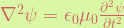

This has the more explicit form: , with  and  SI units and  SI units, we have speed-of-light .

2. From Maxwell equations we can show — eg by assuming harmonic waves — see this and this, that  and fields are transverse in nature.

The details of these on the presumption of harmonic plane waves have been presented here by me, see slides 23 – 27, if you wanna have a look in your leisure.

3. — e.g. . One has to be careful about the exact direction (component) as these are vector quantities and can be both axial or polar vector.

This represents how the magnitudes of the two fields are interdependent. But in reality one must be considerate of their vector nature. So the first of the above equation, (), can be a tad bit misleading, although its true, its true in a  vectorial sense as expressed by the second equation, ().

4. “A wave is nothing if it does not transport energy from one space-time point to another”.

Says a 2 millennia old adage, sure it does not, but now we know its true.

We can get all information of transportation of energy in em waves or light, from the Maxwell’s equations. The energy densities or energy per unit volume, are denoted by a symbol u so that same for electric field  and magnetic field  are given by the respective subscripts,  and .

By using results of 3 above and the fact that speed of light is the inverse of square root of permeability and permittivity of free space, we can easily show that: .

So total energy density carried by the em waves is the sum due to 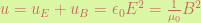 and fields. Thus we have .

If we define S to be the energy per unit time, carried across an unit area of cross section, then considering a cylindrical geometry of energy transport by the em wave we have: .

So we have: .

In general we have S as a vector given by: .

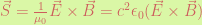
Vector is known as Poynting vector and gives the amount of energy transported by the em waves in an unit time across an unit area, hence its also the power per unit area.

5. Irradiance.

We define irradiance to be the average energy per unit area per unit time, we have already seen how it would look like, in lecture — VII, ( here ) we also called it the radiant flux density.

One can see this as the intensity as well, and evidently its the average of the Poynting vector magnitude over a given time.

Poynting vector gives the instantaneous value of power per area, but irradiance gives the average value, thats the only difference.

For harmonic waves: .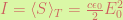

We see that irradiance is proportional to the square of the electric field amplitude.

We can also write the same in terms of instantaneous values of or fields instead of just the amplitude of  or field.

.

For any linear, homogeneous, isotropic dielectric medium, also know as simple media, which is the result we already used in our study of interference in lecture — VII, optics series.