Lectures on Electricity and Magnetism — new series of lectures – EML – 5, 6, 7, 8.
All articles in this series will be found here. Click on link to left or search for menu “E AND M BASICS” on top.
Laplace And Poisson Equation; Boundary Value Problems, Applications And Solved Problems, Lecture 5, 6, 7, 8.
In our last lecture (EML-4) we discussed the conservative nature of the static electric field which also meant such fields are irrotational vector fields (that means their curl is zero). This led us to the formulation of electrostatic potential energy and electrostatic potential. Today we will see how this leads us further and lands us into the land of opportunities where we can solve, using the gained insights and relations a treasure trove of physical problems in electrostatics. We will study few examples of the usefulness of the knowledge we gained so far.
Recapitulation: In our first lecture in this series which can be found here; EML1, we laid a good foundation about the concepts of electric field, lines of force, flux and Gauss Law. In the second one (EML2) we discussed how to apply Gauss Law to find the electric field if cylindrical or planar symmetries are present in the problem, we solved the case of an infinitely long uniformly charged rod and an infinitely large non-conducting sheet of uniform charge. In the 3rd one (and EML3) we discussed how to do the same if spherical symmetry is present e.g. in the case of a spherical shell with uniform charge and a non-conducting spherical solid with uniform charge in its entire body.
+ click to see more about this article
This article belongs to a group of lectures I intend to prepare for their online dissemination — these were delivered in a physical format, beginning with hand written notes that were delivered in a classroom full of students. This series is on Electricity and Magnetism and bears the name sake Electricity and Magnetism Lectures and the number of the lecture will be appended to the end to reflect the same. eg the current lectures will be named EML – 5, 6, 7, 8 . A part of this lecture was delivered to honors students on 10th Feb 2017 and rest were taught later to different classes on 16 and 17th May 2019.
In the meanwhile if you can’t wait and you need some of these concepts at the earliest, here is a slide-share presentation I had made roughly 5 years ago that consists of “some of the things” an undergrad needs: Electricity and Magnetism slides. There are other slides on different topics at that account of mine on slideshare.net (such as; Introduction to Quantum Mechanics , and these are quite well received by the community for their usefulness).
Laplace And Poisson Equation
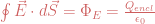
Integral Form Of Gauss Law
We saw in our previous lecture that electrostatic fields can be written as the (negative) gradients of scalar function Φ (called electrostatic potential): 
Gauss Divergence Theorem and Differential Form Of Gauss Law
We will now convert the integral form of Gauss law into its differential form, a veritably useful form at times, where the former won’t do. For this we need the Gauss divergence theorem (Gauss invented all his tools in-house didn’t he?). The Gauss divergence theorem relates the flux of a vector field through a closed surface to the divergence of the field in the volume bounded by the surface, mathematically: 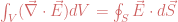
We realize that the total charge enclosed in the volume V is nothing but the volume integral of the volumetric charge density ρ, i.e. 

Poisson Equation
We saw that the consequence of having a conservative vector is that its also irrotational (i.e. its curl is zero), in-fact we mentioned that due to Helmholtz theorem these two facts are concurrent, i.e. one ensures the other. Thus our conservative electrostatic field leads to its curl being zero: 

Laplace Equation
If Φ is considered in a region, where there are no sources of electric charge, the charge density ρ is zero, in such regions. Then Poisson equation becomes the Laplace equation: 
What happens to the curl equation: 

This means the curl equation does not supply anything special or any additional information other than what we already have, viz, the Poisson equation. Why is this so? Because we used the curl equation to find the potential formulation of the electrostatic field so the gradient of that potential merely restates or confirms the curl equation. This is what Helmholtz theorem states, as we have discussed already.
Advantage of Poisson Equation
Poisson equation is a differential equation. It determines Φ which is a scalar field, so only one equation is sufficient. On the other hand E which is a vector field needs two equations, the divergence equation called Gauss law
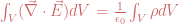
Solution to Poisson Equation
We can find solution to the Poisson equation if we know charge distribution ρ as a function of position. In general: 
Laplace Equation in Spherical Polar Coordinates
Spherical Symmetry
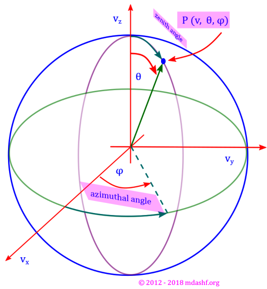
Any problem that involves a spherical symmetry (one where the results don’t change with change in angular direction but changes exclusively with radial distance) entails a spherical polar coordinate system for the easiest analysis. Hence we will cast the Laplace equation into its spherical polar form and suggest its general solutions in terms of Legendre polynomials, before solving some actual problems with spherical symmetry and more. The following diagram shows the spherical polar coordinate system, here v is a vector whose Cartesian values are vx, vy and vz and its spherical polar components are v, θ and φ where v is the magnitude of v.
Laplace equation involves the Laplacian (∇2) and by employing the form of Laplacian in the spherical polar coordinates, we can write the following expression for the Laplace equation for the electrostatic potential Φ: 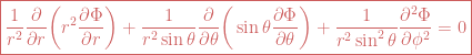
Azimuthal Symmetry
If the problem has azimuthal symmetry i.e. potential Φ does not depend on azimuthal angle φ; Φ(r, θ , φ) = Φ(r, θ), then the spherical coordinate form of the Laplace equation reduces to one that involves differentiation wrt r and θ only and is given by: 
Variable Separable Method
This is amenable to the variable separable method of solving a differential equation. In fact r, θ , φ dependence is also amenable to the variable separable, but now we will deal with the simpler case of r, θ dependence only. We therefore assume a solution in the form of factorizable parts: Φ(r, θ) = R(r) Θ(θ). Following the basic rules of differentiation of a product of a function to a constant factor, we can write: 

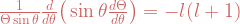
We get: 
We have accordingly: radial part 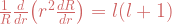
The radial equation is 


Legendre Polynomial
The Legendre Polynomials Pl(x) are defined by the Rodrigue’s formula (with x = cos θ): 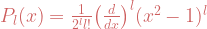


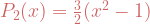


Pl(x) is a lth order polynomial in x, it contains only even powers if l is even and only odd powers if l is odd. 

Boundary Value Problem in Uniform Electric Field.
Now we are in a position to solve boundary value problems. We will illustrate the method in spherical system for the following three problems.
A Simple Spherical Symmetry Problem
Problem 1: For some spherically symmetric distribution of charge, the potential on the surface of a sphere of radius R is given to be V0. Calculate the potential in the region r > R. Also calculate the potential in the region r < R, when no charges are present inside the sphere.
There is spherical symmetry in the problem so potential Φ must depend only on radial distance r and independent of the angular dimensions: θ and φ. As a result: 

This leads to a simpler form for the Laplace equation: 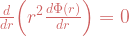

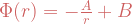
Region I: (i.e. r ≥ R) No charges are present at ∞ so Φ(∞) = 0 ⇒ Φ(∞) = 0 = B. 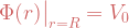
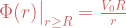
Region II: (i.e. r ≥ R) No charges are present in this region so ⇒ Φ(r) = -A’/r + B’. At r = 0, Φ has to be finite, this is possible if A’ = 0. ⇒ Φ(r) = B’. At r = R, Φ = V0 ⇒ B’= V0. So Φ(r) = V0.
Dielectric Sphere In A Uniform Electric Field
Problem 2: A uniform electric field 

Azimuthal Symmetry
We have azimuthal symmetry due to the sphere and the electric field as the system has axial independence. If we rotate the sphere about z-axis (electric field is aligned along this axis) the result won’t change. That means changing the azimuthal coordinate φ from one value to another won’t change the result, so: Φ(r, θ , φ) = Φ(r, θ). We have seen this above and called this azimuthal symmetry. Hence we can use the results that we derived above.
Application of Solution to Laplace equation; Outside Sphere
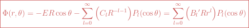
For r > R i.e. outside region of the sphere there are no free charges, hence Laplace equation: ∇2Φ = 0 is satisfied. We have seen above that solution for Laplace equation with azimuthal symmetry is given by: 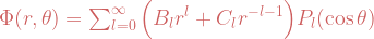
Boundary Conditions
BC 1: All induced charges are at finite values of r hence introduction of the dielectric sphere won’t change the existing uniform field 


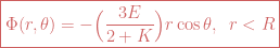
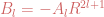
Lets apply this boundary condition to the general solution to Laplace equation. We get: B1 r cos θ = -E r cos θ. We see that r-l-1 = 0 if r → ∞ and l = 1 gives non-zero Bl, Bl = 0 if l ≠ 1 so B1 = -E. Thus the solution looks like: 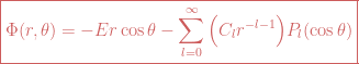
Lets apply boundary conditions inside of the dielectric sphere (and on it), i.e. r ≤ R, there are no free charges, Laplace equation is satisfied, like before. But the solution to the Laplace equation now is given by a new set of constants Bl‘ and Cl‘. Solution for r < R; 
BC2: At origin (r = 0) the potential must be finite as there are no point charges there, this means Cl‘ for all l must be set to zero.
BC3: The potential must be continuous across r = R, i.e. across the surface of the spherical dielectric material, due to absence of free charges. So the solution for r > R that we obtained and the one we obtained above for r ≤ R must be set equal.
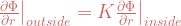
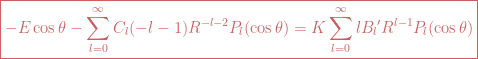
BC4: We know the boundary conditions to be imposed on fields when they pass through material media, and we have discussed this here. We will use that result by remembering that normal vector component of the vector D is continuous across boundary r = R as there are no free charges at that interface. i.e. 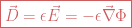
Orthogonality Properties of Legendre Polynomials: The Legendre Polynomials satisfy the following orthogonality and normality properties: 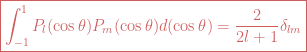


Now we multiply eqn-1 by (-m-1) and eqn-2 by R and subtract, to get; 
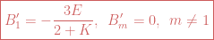

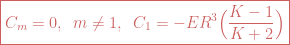
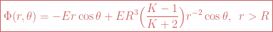
We now have all the required constants and so the solutions for the electrostatic potential for the given problem, both inside and outside the dielectric sphere.


Uncharged Metal Sphere In A Uniform Electric Field
Problem 3: An uncharged metal sphere of radius R is placed in an otherwise uniform electric field 

The field will push positive charge to the upper i.e. northern surface of the sphere and negative charges will be pushed to the lower or southern surface. The surface of the sphere is an equipotential surface (as metals are conductors). We can choose this equipotential value to be zero.
The potential Φ does not go to zero for large values of z. Far from the sphere, field is 
The boundary conditions are
- i. Φ = 0 when r = R.
- ii. Φ→ -E0r cos θ, for r >> R
Solution: We have seen that our general solution has the form: 


Induced Charge Density: Now we can give a word about the induced charge density: 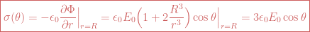
Now we will turn our gaze into a problem with a different symmetry than spherical or azimuthal symmetry. Sometimes we need to employ both Laplace and Poisson equation in a given problem. The following is an example.
Infinite Planar Symmetry
Problem 4: Let A, B, C and D be infinite planar surfaces. A and D are at zero potential. Region between B and C has charges with a constant charge density ρ. The separation between A and B, between B and C and between C and D are d, 2t and d respectively. Calculate the electrostatic potential between A and B, between B and C and between C and D.
We begin with the following simple diagram that represents the situation.

The normal to the surfaces is along z-axis, mid point between B and C is at z = 0. The potential depends only upon z (due to planar symmetry it does not depend upon x and y). Let V1, V2 and V3 be the potential between A & B (region 1), between B & C (region 2) and between C & D (region 3) respectively. Lets use the Cartesian coordinate system, where Laplacian has the following form: 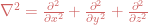
The potential equations are either Laplace equation or Poisson equation: 


To find their solutions we integrate each equation, and obtain: V1 = C1z + C2, V2 = C3z + C4 – 4πkρz2/2 and V3 = C5z + C6. According to the boundary value conditions at z = d + t and z = -d – t the potential is zero at these surfaces. This gives C2 + C1(d + t) and C6 + C5(-d – t). Thus V1 = C1(-z -d -t) and V3 = C5(z + d + t).
Another boundary value condition is at z = t the potentials are continuous so V1 = V2 and 

Solutions For The 3 Potentials: Now we can solve for the constants C1, C3, C4 and C5 by elimination. We eliminate C1 from first two equations, and C5 from last two equations. We obtain: C3(t + d) + C4 = 4πkρ(t2/2 + td) and C3(t + d) – C4 = -4πkρ(t2/2 + td). This gives us C3 = 0, C4 = 4πkρ(t2/2 + td), C1 = -4πkρt and C5 = 4πkρt. Thus we have the 3 solutions given by: V1 = -4πkρt(z – d – t), V2 = 4πkρt(t/2 + d) – 4πkρz2/2, V3 = 4πkρt(z + d + t).
Solved Problems on Boundary Value Conditions and Laplace/Poisson Equation.
Now we will solve a few boundary value problems on the Laplace and Poisson equation before wrapping up this longish lecture. Aptly 4 lecture hours has been devoted to this article, but it helps to put certain things together.
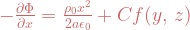
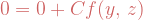
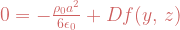
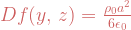
Problem 5: In a one dimensional device the charge density is given by, ρv = ρ0x/a. If E = 0 at x = 0 and V = 0 at x = a, find V and E using Poisson Equation of electrostatics.
In 1 dimension the Poisson’s equation takes the form: 

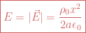
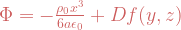
We integrate the above solution for electric field once again to get the electrostatic potential: 

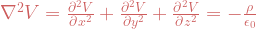
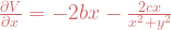
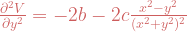
Problem 6: What is the volume density of charge in a region of space where electrostatic potential is given by V = a – b(x2 + y2) – c log (x2 + y2), where a, b, c are constants?
The Poisson equations reads as: 


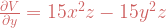
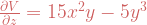
Problem 7: Verify whether the electric potential V = 15x2yz – 5y3z, satisfies Laplace equation or not?
Laplace equation in Cartesian coordinate system reads as: 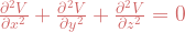


Leave a comment