
Electromagnetic theory, lecture — III.
Helmholtz theorem. Vector and Scalar Potentials.
This lecture, the web version of the third lecture given in the electromagnetic theory paper of the physics honors degree class, was delivered on 9th January 2018.
All electromagnetic theory lectures of this series, will be found here.

Topics covered
A. Formalism of electrodynamics — fundamental theorem
B. Application of Helmholtz theorem — to electrostatics
C. Application of Helmholtz theorem — to magnetostatics
Formalism of electrodynamics
Helmholtz theorem
In our previous lectures, lecture – I and lecture — II, we discussed the Maxwell’s equations in free space and in material media. We also discussed the boundary conditions which helps us solve for the 

The 

The Helmholtz theorems provides some useful relations and properties which helps us determine the
One needs a basic proficiency in vector calculus to be able to grasp the inherent significance of these methods. To begin with one can go through the slides here — vector calculus, to have a reasonable hold on the vector calculus concepts.
There is a theorem which deals with the implications of curl of a vector.
Theorem 1
If curl of a vector field is zero — everywhere, then 


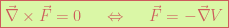
Here the minus sign is just a convention.
a. Such fields, —
b. The curl is zero everywhere. I.e.

c. The quantity 


d. The quantity 
e. The vector 
f. If any one of the above statement is valid, it ensures all the others to be valid. That implies 
g. Scalar potential

Now there is a theorem which deals with the implications of divergence of a vector.
Theorem 2
If divergence — 
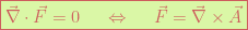
a. Such fields —
b. The divergence is zero everywhere. I.e. 
c. The quantity 
d. The quantity 
e. The vector 
f. If any one of the above statement is valid, it ensures all the others to be valid. That implies 
g. Vector potential 
I.e. if 

There is another mathematical result which has implications for both of the above theorems and we will state it.
Any general vector irrespective of whether this vector is divergence-less or not, and whether this vector is curl-less or not, can always be written as the sum of two vectors,
a. one vector which is the curl of some vector and
b. another vector which is the divergence of some scalar function.
In symbols: 
Application of the above theorems to 3 situations
We will study how the above theorems have a great deal of implication for almost all of the field of electromagnetic theory. These theorems are together known as Helmholtz theorems.
But we will study them under 3 situations — gradually moving up the ladder of generality, beginning with our familiar knowledge of the static electric and magnetic fields.
a. Electrostatics
b. Magnetostatics
and
c. Electrodynamics
Electrostatics
When electric charges are stationary the resulting electric fields lead to electrostatic behavior. Under these conditions, electric fields —
Because 
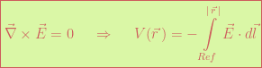
Here Ref — for reference, on the lower limit of the integral sign stands for a particularly chosen location for the potential, from where all calculations are to be made. There are two standards for this idea to be implemented;
a. if charge distributions are finite, reference can be set to
b. if charge distributions are not finite, other means are to be explored to calculate 

The above boxed equation which we can define because curl of the electrostatic field

In the electrostatics conditions, the potential formulation serves a very useful role, as 1 scalar equation is to be solved in lieu of 3 vector equations — we do not have to bother about the 3 vector components, which makes the problem cumbersome.
The two Maxwell equations — one vector and one scalar, 

Poisson’s equation:

When source term is absent i.e. 
Laplace equation:

Potential can now be calculated as:
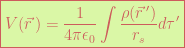
where 


Magnetostatics
Magnetostatics problems follow a similar logic. The magnetostatic nature is defined by stationary currents or steady-currents. That means charge densities that produce the field must not vary in time.
Mathematically: 


The second Maxwell equation is: 
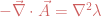
According to theorem 2 of Helmholtz theorem then, magnetic field can always be written as curl of a vector potential 
By Ampere’s law of Maxwell equations — i.e. 

We already discussed that the magnetic vector potential
By this freedom we can always find scalar 


Thus, 

For 
Remember Poisson’s equation for electrostatics: 


As in the case of electrostatics case if 

This solution is given by:
If the source term 
It is always possible to find
Thus Ampere’s law becomes: 
If 

Thus for steady currents we have:

We will discuss the 3rd situation of applicability of the Helmholtz theorems to the most general case of electrodynamics in the next lecture, — lecture — IV.

Leave a comment