Helmholtz theorem in electrodynamics, Gauge transformation.

Electromagnetic theory, lecture — IV

Helmholtz theorem in electrodynamics and gauge transformation

This article has 2184 words — considering latex images to be anywhere between 2 – 40 words.

This lecture, the web version of the 4th lecture given in the electromagnetic theory paper of the physics honors degree class, was delivered on 9th January 2018.

All electromagnetic theory lectures of this series, will be found here.

Topics covered in this lecture

a. Helmholtz theorem — in the formalism of electrodynamics

b. Gauge transformation — of scalar and vector potential in electrodynamics

c. Coulomb and Lorentz gauge — two specific conditions under which gauge transformation can be implemented

In our previous lecture — lecture — III, we discussed in quite detail, the problem of electrostatics and magneto-statics. We understood how deeply the Helmholtz theorems formulate the entire question of these two branches of electromagnetic phenomena.

But static problems are not sufficient for any rigorous treatment of the electromagnetic theory. We promised in that lecture to study how Helmholtz theorems lend their magical power to understand the most general nature of electromagnetic phenomena.

In this lecture we will study precisely the applicability of Helmholtz theorems to the problem of electrodynamics. We will see how it leads to a great deal of success in advancing the ability to solve electromagnetic problems of a great variety.

Helmholtz theorem — in electrodynamics

In electrodynamics the sources of charge and currents are no more stationary. They are now stated by simple relations, $\vec{\nabla}\cdot\vec{j}\neq 0$ and $\frac{\partial \rho}{\partial t}\neq 0$ .

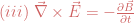
According to the Maxwell’s equations curl of E — i.e. $\vec{\nabla} \times \vec{E}$ , is no more zero. Now the fields are no more stationary, that is the fields vary with time, in magnitude and in direction.

The variation of the $\vec{B}$ field produces a time-varying non-conservative, rotational $\vec{E}$ field while the variation of the $\vec{E}$ field produces a time varying magnetic field $\vec{B}$ .

The $\vec{E} \,\& \,\vec{B}$ fields are no more independent of each other, as they are in the case of static conditions. We sum this by saying the situation as electrodynamics.

Lets write out the Maxwell’s equations;

$(i)\,\,\vec{\nabla}\cdot\vec{E}=\frac{\rho}{\epsilon_0}$

$(ii)\,\,{\vec{\nabla}\cdot\vec{B}=0}$

$(iii)\,\, \vec{\nabla}\times\vec{E} = -\frac{\partial \vec{B}}{\partial t}$

$(iv)\,\,\vec{\nabla}\times\vec{B} =\mu_0\vec{j}+\mu_0 \epsilon_0 \frac {\partial \vec{E}}{ \partial t}$

Since the $\vec{E}$ field is no more a curl-less field according to Helmholtz theorem that we studied in the last lecture ( lecture — III ), we don’t have a scalar potential $V$ that satisfies the form, $\vec{E}=-\vec{\nabla}V$ .

But $\vec{\nabla}\cdot\vec{B}=0$ is always true, in static as well as electrodynamics conditions, so we can apply theorem-2 of Helmholtz theorems and have a magnetic vector potential, $\vec{A}$ that satisfies the form: $\vec{B}=\vec{\nabla}\times\vec{A}$ .

Lets see what we obtain when we use this result with the 3rd equation of Maxwell equations, viz. Faraday’s law — of electromagnetic induction. We get: $\vec{\nabla}\times\vec{E} = - \frac{\partial }{\partial t}(\vec{\nabla}\times \vec{A} )$ , or;

$\boxed{\vec{\nabla}\times\Bigg(\vec{E}+\frac{\partial \vec{A}}{\partial t}\Bigg) = 0\hspace{15pt} eq^n (1)}$

Thus we see that the term in the parenthesis $\vec{E}+\frac{\partial \vec{A}}{\partial t}$ can be written as the gradient of a scalar potential — as dictated by theorem 1 of Helmholtz theorems, so, $\vec{E}+\frac{\partial \vec{A}}{\partial t} = - \vec{\nabla}V$ . Thus the $\vec{E}$ field can now be given as:

$\boxed{\vec{E}= - \vec{\nabla}V- \frac{\partial \vec{A}}{\partial t}\hspace{15pt} eq^n (2)}$

Let us now use $eq^n \,\,(2)$ along into $eq^n \,\,(i)$ . That is, the new definition of electric field, according to Helmholtz theorem, in electrodynamics conditions, into Gauss law in Maxwell’s equation $(i)$ . We obtain $eq^n\,\,(3)$ .

$\boxed{ \nabla^2 V + \frac{\partial}{\partial t}(\vec{\nabla}\cdot\vec{A})=-\frac{1}{\epsilon_0}\rho \hspace{15pt}eq^n\,\,(3)}$

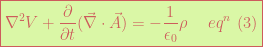
We see that instead of Poisson’s equation we have obtained a bit more nuanced equation, that would reduce to the Poisson’s equation only under special conditions. A Poisson’s equation ensures an easy way for a solution to the differential equation, but we will worry about it a little later.

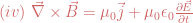
Now let us use the magnetic field $\vec{B}$ in terms of the vector potential $\vec{A}$ i.e. — $\vec{B} = \vec{\nabla}\times\vec{A}$ , and $eq^n \,\,(2)$ into $eq^n \,\,(iv)$ of the Maxwell’s equation, i.e. Ampere-Maxwell relation, or modified Ampere’s law: $\vec{\nabla}\times\vec{B} =\mu_0 \vec{j}+\mu_0 \epsilon_0\frac{\partial \vec{E}}{\partial t}$ .

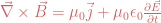
We obtain: $\vec{\nabla}\times(\vec{\nabla}\times\vec{A})=\mu_0\vec{j} - \mu_0 \epsilon_0 \vec{\nabla}\big(\frac{\partial V}{\partial t}\big)-\mu_0 \epsilon_0 \frac{\partial ^2 \vec{A}}{\partial t^2}$ . Lets use the vector identity: $\vec{\nabla}\times(\vec{\nabla}\times\vec{A})=\vec{\nabla}(\vec{\nabla}\cdot\vec{A})-\nabla^2 \vec{A}$ , and rearrange terms on both sides.

We have now:

$\boxed{\Bigg(\nabla^2 \vec{A} - \mu_0 \epsilon_0 \frac{\partial ^2 \vec{A}}{\partial t^2}\Bigg) - \vec{\nabla}\Bigg(\vec{\nabla}\cdot\vec{A} + \mu_0 \epsilon_0 \frac{\partial V}{\partial t}\Bigg) = -\mu_0 \vec{j}\hspace{15pt}eq^n\,\,(4)}$ .

Thus now we have all the information of the 4 Maxwell’s equations transferred to 2 equations viz. $eq^n (3) \,\, \& \,\,eq^n (4)$ .

But these two equations look formidable, don’t they? Like difficult people we need to formulate strategies to deal with difficult equations as well — and fortunately its possible in most daunting situations that we can find ways around them.

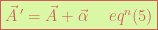
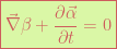
The advantage is that the problem of finding 6 solutions — 3 for the $\vec{E}$ field and 3 for the $\vec{B}$ field, has reduced to finding only 4 solutions — 1 for the scalar potential $V$ and 3 for the vector potential $\vec{A}$ .
$eq^n (3) \,\, \& \,\,eq^n (4)$ do not have unique solutions.
$\vec{A} \,\,\&\,\,V$ are quite arbitrary. we can chose them to make $eq^n (3) \,\, \& \,\,eq^n (4)$ as easy as satisfies us, while it is still possible.

This freedom of choosing our scalar and vector potentials is whats known as “Gauge freedom” and the resulting possible transformations of $(V\,\, \& \,\,\vec{A})$ from one set to another is known as “Gauge transformation“.

Now let us study the behavior of Gauge transformation in electrodynamics. We are still going to be indebted to the help Helmholtz theorem is going to extend in our quest to find the $\vec{E}\,\,\&\,\,\vec{B}$ fields, by first finding the vector and scalar potentials $\vec{A} \,\,\&\,\,V$ .

Gauge transformation of scalar and vector potentials

Let us now see how two sets of scalar — $V$ , and vector — $\vec{A}$ , potentials are related to each other.

Lets write

$\boxed{\vec{A}\,' = \vec{A} + \vec{\alpha} \hspace{15pt} eq^n (5)}$

and

$\boxed{V\,' = V + \beta \hspace{15pt} eq^n (6)}$

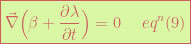
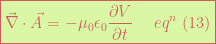
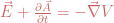
As we know already, the gauge transformation should lead to the same field vectors, so, $(\vec{A} \,\,\&\,\,\vec{A}\,')$ must give rise to the same $\vec{B}$ field.

Thus $\boxed{\vec{\nabla}\times\vec{\alpha}=0\hspace{15pt} eq^n (7)}$ .

This is where we need to be thankful of the Helmholtz theorems, because the curl-less vector — $\vec{\alpha}$ , can be expressed as the gradient of a scalar function, according to the theorem-1 of the Helmholtz theorems:

$\boxed{\vec{\alpha} = \vec{\nabla} \lambda\hspace{15pt} eq^n (8)}$ .

Also the two scalar potentials $(V\,\, \& \,\,V\,')$ must give rise to the same $\vec{E}$ field.

This necessitates:

$\boxed{\vec{\nabla}\beta+\frac{\partial \vec{\alpha}}{\partial t}=0}$

$\boxed{\vec{\nabla}\Big(\beta+\frac{\partial \lambda}{\partial t}\Big)=0\hspace{15pt} eq^n (9)}$ .

$eq^n (9)$ means $\beta+\frac{\partial \lambda}{\partial t}$ is independent of “position” but it can depend on “time“: $\beta = -\frac{\partial \lambda}{\partial t} + K(t)$ .

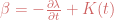
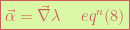
We can redefine $\lambda$ by adding $\int\limits_0^t K(t\,') dt\,'$ to $\lambda$ ; but $\vec{\nabla}\lambda$ is unaffected. Only $K(t)$ is added to $\frac{\partial \lambda}{\partial t}$ .

Thus

$\boxed{\vec{A}\,' = \vec{A} + \vec{\nabla} \lambda \hspace{15pt} \& \hspace{15pt} V\,' = V- \frac{\partial \lambda}{\partial t}\hspace{15pt}eq^n (10)}$ .

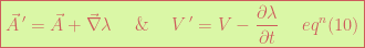
Thus adding $\vec{\nabla}\lambda$ to $\vec{A}$ we must at the same time subtract $\frac{\partial \lambda}{\partial t}$ from $V$ . It does not alter $\vec{E}$ or $\vec{B}$ .

Expressions in $eq^n (10)$ are known as Gauge transformations. With these changes now we can alter $\vec{A}\,\,\&\,\,V$ appropriately to easily work out solutions to Maxwell’s equations.

Coulomb and Lorentz gauge

There are two specific types of Gauge freedom that we will discuss in particular.

(i) Coulomb Gauge

and

(ii) Lorentz Gauge

Coulomb Gauge

In our discussion for magnetostatics we saw that $\vec{\nabla}\cdot\vec{A}=0$ allowed us to solve Poisson’s equation and hence determine $\vec{B}$ which led to the Biot-Savart’s law.

In electrodynamics also we can employ the same condition to our advantage.

$\vec{\nabla}\cdot\vec{A}=0$ leads to $\nabla^2 V = -\frac{1}{\epsilon_0}\rho$ — from $eq^n (3)$ — i.e. from $\nabla^2 V + \frac{\partial}{\partial t}(\vec{\nabla}\cdot\vec{A})=-\frac{1}{\epsilon_0}\rho$ .

If $V=0 \,\,\,at\,\,\,\infty$ we can solve the above — i.e. the Poisson’s equation, and find $V$ .

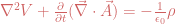
As in the case of electrostatics we have a Coulomb’s law like potential from the external form.

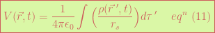
$\boxed{V(\vec{r}, t) = \frac{1}{4\pi\epsilon_0}\int \Big(\frac{\rho(\vec{r}\,',t)}{r_s}\Big)d\tau\,'\hspace{15pt}eq^n \,\,(11)}$ ,

remember from our last lecture the definition of the separation vector 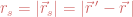$r_s =|\vec{r}_s|=|\vec{r}\,'-\vec{r}\,|$ .

But looks can be deceptive — this is not the $V$ which determines the field $\vec{E}$ in a straight forward way, as a scalar potential whose gradient is $\vec{E}$ . We are now in whirlpool and there is a feedback between $\vec{E}$ and $\vec{B}$ , which means a feedback between $V$ and $\vec{A}$ .

We need to know $\vec{A}$ in order to be able to determine $\vec{E}$ .

The advantage of Coulomb gauge is it is easier to calculate the scalar potential $V$ , as in the case of electro- or magneto- statics.
The disadvantage in this gauge is it is still difficult to determine the vector potential $\vec{A}$ .

Now the differential equation for $\vec{A}$ is dependent upon the solution for $V$ . By using the Coulomb gauge — $\vec{\nabla}\cdot\vec{A}=0$ , in $eq^n\,\,(4)$ we have a solution for $\vec{A}$ only in terms of $V$ .

$\boxed{\nabla^2 \vec{A}-\mu_0 \epsilon_0 \frac{\partial ^2 \vec{A}}{\partial t^2}=-\mu_0 \vec{j} + \mu_0 \epsilon_0 \vec{\nabla} \Big( \frac{\partial V}{\partial t}\Big)\hspace{15pt}eq^n \,\,(12)}$

i.e. $eq^n \,\, (12)$ has to be be solved using $eq^n\,\,(11)$ .

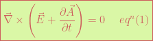
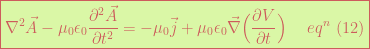
Lorentz gauge

We choose our $\vec{A}\,\,\&\,\,V$ so that they satisfy:

$\boxed{\vec{\nabla}\cdot\vec{A}=-\mu_0 \epsilon_0 \frac{\partial V}{\partial t}\hspace{15pt}eq^n \,\,(13)}$ .

This boxed condition is known as Lorentz gauge. Thus $eq^n\,\,(3) \,\,\&\,\,eq^n\,\,(4)$ are now simplified to 2 equations, whose form is the same, in terms of the differentiation operation.

We obtain:

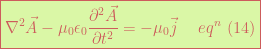
$\boxed{\nabla^2 \vec{A} - \mu_0 \epsilon_0 \frac{\partial ^2 \vec{A}}{\partial t^2}=-\mu_0 \vec{j}\hspace{15pt}eq^n \,\,(14)}$

and

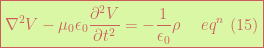
$\boxed{\nabla^2 V - \mu_0 \epsilon_0 \frac{\partial ^2 V}{\partial t^2}=-\frac{1}{\epsilon_0}\rho \hspace{15pt}eq^n \,\,(15)}$

Now both the scalar potential $V$ and the vector potential $\vec{A}$ are on equivalent status. The two equations above both have the differentiation operator $\Box^2 = \nabla^2 - \mu_0 \epsilon_0 \frac{\partial ^2}{\partial t^2}$ and this operator is known as d’ Alembertian.

It treats both scalar and vector potentials equivalently and we have: $\Box^2 V=-\frac{1}{\epsilon_0}\rho$ and $\Box^2 \vec{A}= -\mu_0 \vec{j}$ .

These are the 4-dimensional equivalent of Poisson’s equation. In the Lorentz gauge the wave equation looks like $\Box^2 f = 0$ and $V\,\,\&\vec{A}$ satisfy the “inhomogeneous wave equation” with $\rho\,\,\&\,\,\vec{j}$ as the source terms.

3 thoughts

Pingback: Helmholtz theorem. Scalar and vector potentials – M Dash Foundation
Pingback: Interference of two plane harmonic waves – M Dash Foundation
Pingback: Conservative Nature of the Electrostatic Field and Electrostatic Potential, Lecture – 4. – M Dash Foundation: C Cube Learning

M Dash Foundation: C Cube Learning

Invariance: A journal with a difference, where mind meets aspiration

Helmholtz theorem in electrodynamics, Gauge transformation.

Electromagnetic theory, lecture — IV