Conservative Nature of the Electrostatic Field and Electrostatic Potential, Lecture – 4.

Lectures on Electricity and Magnetism — new series of lectures – EML – 4.

All articles in this series will be found here. Click on link to left or search for menu “E AND M BASICS” on top.

Conservative Nature of the Electrostatic Field and Electrostatic Potential Lecture – 4.

In our first lecture in this series which can be found here; EML1, we laid a good foundation about the concepts of electric field, lines of force, flux and Gauss Law. In the second one (EML2) we discussed how to apply Gauss Law to find the electric field if cylindrical or planar symmetries are present in the problem, we solved the case of an infinitely long uniformly charged rod and an infinitely large non-conducting sheet of uniform charge. In the 3rd one (and EML3) we discussed how to do the same if spherical symmetry is present e.g. in the case of a spherical shell with uniform charge and a non-conducting spherical solid with uniform charge in its entire body.

Today we will discuss the conservative nature of the static electric field — the time varying fields are not amenable to this conservative nature as we would learn in an advance discourse. This is intimately connected with the concept of the Helmholtz theorem which has been discussed on this website (linked below), in an advance course called Electromagnetic Theory, suitable for the senior Honors student.

The Helmholtz theorems are a great framework of almost all of Electrodynamics and sooner or later a serious student of Physics must master them. Here are two lectures that covers the theorem in good detail ETL-3 and ETL-4 (albeit technical language can often not be traded with lucid discourse, at-least in its first attempt). Anyone who is comfortable with the advance nature of those lectures is welcome to lay his/her sight on them after reading this basic discourse.

Its the conservative nature of electrostatic field which leads to the most important concept of the electrostatic potential (and electrostatic potential energy) which we will also discuss in this lecture.

+ click to see more about this article

This article belongs to a group of lectures I intend to prepare for their online dissemination — these were delivered in a physical format, beginning with hand written notes that were delivered in a classroom full of students. This series is on Electricity and Magnetism and bears the name sake Electricity and Magnetism Lectures and the number of the lecture will be appended to the end to reflect the same. eg the current lecture will be named EML – 4 . This lecture was delivered to honors students on 9th Feb 2017.

In the meanwhile if you can’t wait and you need some of these concepts at the earliest, here is a slide-share presentation I had made roughly 5 years ago that consists of “some of the things” an undergrad needs: Electricity and Magnetism slides. There are other slides on different topics at that account of mine on slideshare.net (such as; Introduction to Quantum Mechanics , and these are quite well received by the community for their usefulness).

Conservative Nature of the Electrostatic Field

Electrostatic field E and corresponding electric force F are vector fields (you can learn some important facts about vector fields here). The E and F vectors have 3 vector components each, and its considerably more complicated to calculate or compute solutions involving them.

But fortunately there are scalar fields corresponding to these vector fields which make things easier. The corresponding scalar fields to E and F vector fields are known as electrostatic potential and electrostatic potential energy. These scalar fields are convenient because the vector fields are conservative in nature i.e. electrostatic work done in moving a charge from one point to another in these fields is independent of path followed, it depends only upon end points of the path taken.

Lets check this property of the work done in electrostatic fields in two different situations. Because of electrostatic work’s independence from path followed we can define scalar fields which are known as electrostatic potential; and electrostatic potential energy based on this work.

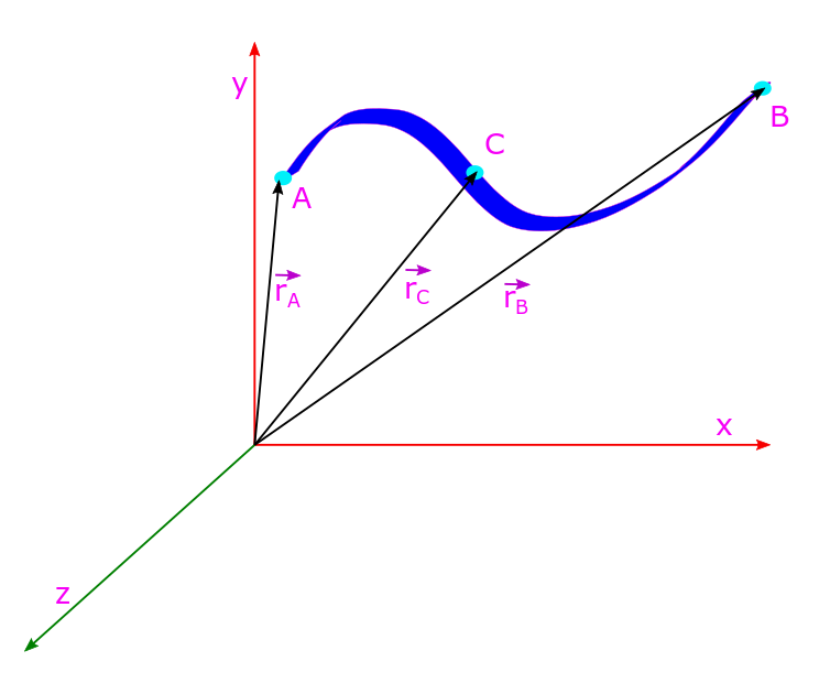
For the above purpose lets consider the following diagram.

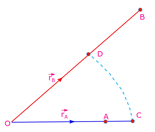
Let A and B be two positions in the electrostatic field of charge Q, located at the origin O. Their position vectors are r_A and r_B. Let a charge move from point A to point C and from point C to point D. Then it moves from point D to point B. AC and DB are radial paths, along vectors r_A and r_B and respectively, but CD is an arc centered at O.

The electrostatic force at (position vector) r is given by Coulomb’s law: . Here q is the test charge that we wanna move around in the field of source charge Q.

Note: In order to impart zero acceleration to move this charge, i.e. to move the charge under uniform motion, one must exert an equal and opposite force to the electrostatic Coulomb force experienced by the charge q, that is the whole idea why we must calculate work done due to this Coulomb force, and the work done by this external agent in keeping the charge evade acceleration, is stored as the potential energy in the electrostatic system, and thats why there is a -ve sign in front of the work done, because the actual force exerted to keep the charge under uniform motion is opposite to the Coulomb’s force and its the latter which we are using in the work-expression. Thus; .

Lets now calculate the work done in moving charge q along path ABCD; .

Similarly: .

But W_CD = 0 as electric field is radial and perpendicular to the arc which is the path of the charge’s motion. Thus since r_D = r_C. Hence work done is independent of the particular path followed here, it depends only upon end points A and B.

We can also show that work done against electrostatics force (which as we mentioned above is equal and opposite to the work done by this electrostatics force) is independent of any arbitrary path followed between end points and depends only upon these end points. Thus electrostatic forces are conservative forces and electrostatic fields are known as conservative fields.

Irrotational nature of electrostatic field

There is an important consequence of this. The work done by an electrostatic force is the line integral of the force F along this path. Thus the line integral of F and E can be converted into integrals in terms of curl of these vectors. (By the well known Stoke’s integral theorem: e.g. .)

The line integral is zero for closed loops for conservative vectors, (here C stands for contour = loop) and this leads to the fact that curl of the vectors is identically zero. Such vectors whose curl is zero (F and E) are known as “irrotational vectors” apart from being “conservative vectors”. This is one of the result of one part of the Helmholtz theorem that we mentioned and linked in the beginning. (There are two parts of this theorem, if you follow the link: ETL-3, and for logical conclusion you can also read through ETL-4.)

Let us see how our above assertion can be proved. The Helmholtz theorems are more nuanced and involved, but this one serves to strike the right chord if you are beginning to appreciate the elegance and power of vector methods in electrostatics. Lets consider the following simple diagram which shows a closed loop traversing through points P, S, R and T.

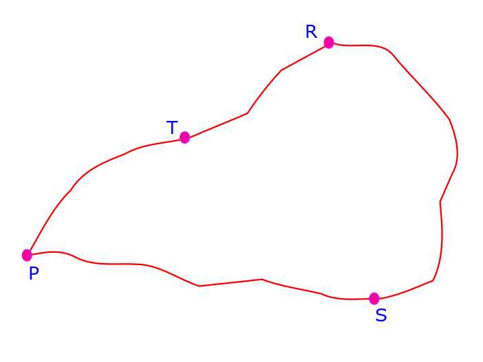
Let the test charge q move along a loop (as shown) PSRTP, then the line integral of the electric field can be decomposed into the following parts — which is a purely mathematical step following the rules of usual integration: .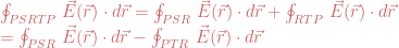

We can now use the Stoke’s theorem that we mentioned above: . Here A is the surface bounded by the loop PSRTP (hence its an open surface).

If LHS is zero, so is RHS and this translates to for all points. In a more general prospective, if N point charges are located at position vectors R_i, where the index i runs from 1 to N, the field at the reference point P(r) is given by: .

Homework: by showing that prove that: , for the above expression of electric field.

According to Helmholtz theorem the reverse of the above result is also true, i.e. if a vector is irrotational its necessarily conservative. All this is valid in electrostatics though. Now we are in a position to delve into the concept of the electrostatics potential which follows from the concept of electrostatics potential energy. As we mentioned in the beginning this follows from the conservative (or equivalently irrotational) nature of the electrostatics vector fields F and E.

Electrostatic Potential

Lets consider the above diagram. Let the test charge q (a point, unit and positive charge) move from point A to point B via point C. Since line integrals of the force vector over any path can be written as sum over various parts of the consecutive path (which is a purely mathematical license) the total work done can also be written as sum over these respective paths. So we can write: .

Point C is arbitrary and work done in moving charge from A to B does not depend on C. This is possible if there exists functions, Φ such that: and , i.e. a function Φ which gives work W as a value that depends only on end points and not intermediary points. We see that Φ(r_C) cancels out in calculating giving: .

The scalar Φ(r) is called as electrostatic potential. Note that since we have taken the test charge to be of unit magnitude electrostatic potential and electrostatic potential energy are synonymous and equal to the work done against the Coulomb’s force to move the charge between specified points. But in general the work done against the Coulomb force is equal to the potential energy which in turns equals to the charge times the potential. Since work done is independent of path followed difference of potential between two points has any physical meaning, absolute potential has none.

We can define potential at r = ∞ to be zero if all charges are located within finite distances: W(∞, r) = Φ(r) – Φ(∞) = Φ(r). Thus potential at r is defined as the work done in carrying the charge (in uniform motion all along) from infinite distance to the said location r.

So potential (as is work done) is the line integral of the electric field (or in case of work the line integral of the electrostatic force vector). Lets now see the reverse relation i.e. how the electric field (or force) is given as a derivative of the potential (or potential energy).

For this lets consider the charge q when it moves from x to x+dx. In this case for the unit charge the work done is given as -E_xdx (we have confined our attention to the x-direction only). Thus: -E_x(r)dx = Φ(x+dx,y,z) – Φ(x,y,z) = -[∂Φ(r)/∂x]dx ⇒ E_x(r) = –∂Φ/∂x. Similarly we have: E_y(r) = -∂Φ/∂y. and : E_z(r) = -∂Φ/∂z. These 3 expressions are actually what constitutes the vector relationship between electrostatic field E and gradient vector of the electrostatic potential Φ: .

In words we say; the electrostatic field at any point is the negative gradient of the scalar potential at that point, as is the scalar potential the line integral of the electrostatic field. This is to be expected since integral and derivative are inverse relations.

One important concept to remember regarding the potential is the superposition principle according to which potential due to separate charges is the summation of potential due to each charge.