Electrostatic Potential Energy Of Different Charge Configurations. Lecture-10, 11.

Lectures on Electricity and Magnetism — new series of lectures – EML – 10, 11.

All articles in this series will be found here. Click on link to left or search for menu “E AND M BASICS” on top.

Electrostatic Potential Energy Of A System Of Charge, A Charged Sphere And A Conducting Solid Sphere, Lecture-10, 11.

Definition Of Potential energy Of An Electrostatic Distribution Of Charges

We assume the charges to be located infinitely away from each other, initially. The charges interact among each other electrically when they come closer together, by the dint of Coulomb’s force. This gives rise to an electrostatic force between each pair of charge. When the charges come closer we have to perform work against the Coulomb’s force of interaction — eg to move a unit positive test charge in their electrostatic field, at a uniform pace in infinitesimally short straight paths.

Electrostatic Potential Energy of a distribution of electric charges is then defined as the amount of electrostatic work done in assembling the distribution from their elements assumed to be located at infinity.

Previously we have discussed the concept of electrostatic potential energy and electrostatic potential for simple electrostatic charge distributions here and here. In this lecture we will take it up a notch and discuss advanced cases and evaluate their electrostatic potential energy for the following cases:

for a system of charges
for uniformly charged sphere and
for a conducting solid sphere.

+ click to see more about this article

This article belongs to a group of lectures I intend to prepare for their online dissemination — these were delivered in a physical format, beginning with hand written notes that were delivered in a classroom full of students. This series is on Electricity and Magnetism and bears the name sake Electricity and Magnetism Lectures and the number of the lecture will be appended to the end to reflect the same. eg the current lectures will be named EML – 10, 11 . These lectures were delivered to honors students on 20th Feb 2017. The last part of the lectures was delivered to a different class on 18th May 2019.

In the meanwhile if you can’t wait and you need some of these concepts at the earliest, here is a slide-share presentation I had made roughly 5 years ago that consists of “some of the things” an undergrad needs: Electricity and Magnetism slides. There are other slides on different topics at that account of mine on slideshare.net (such as; Introduction to Quantum Mechanics , and these are quite well received by the community for their usefulness).

Electrostatic Potential Energy Of A System Of Discrete Charge

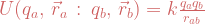
Electrostatic Potential Energy Of A Pair Of Charge

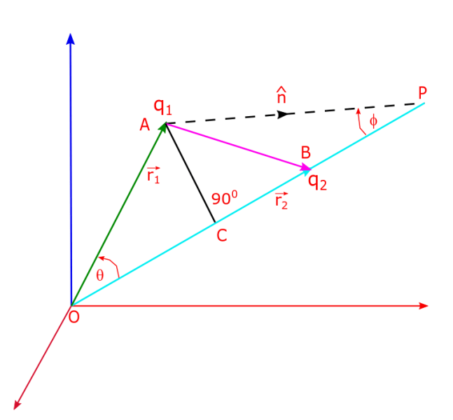
Lets first derive the electrostatic potential energy for two point charges q₁ and q₂ which are located at points given by position vectors r₁ and r₂. Lets consider the following diagram which aptly depicts the situation.

Two point charges q1 and q2 which are located at points given by position vectors r1 and r2. We would like to calculate their potential energy due to electrostatic interaction between them by Coulomb's force. — Two point charges q₁ and q₂ which are located at points given by position vectors r₁ and r₂. We would like to calculate their potential energy due to electrostatic interaction between them by Coulomb’s force.

The potential energy of this simple system can be equivalently determined by two methods;

Keep q₁ fixed at position given by vector r₁ and bring q₂ from ∞ to position given by vector r₂.
Keep q₂ fixed at position given by vector r₂ and bring q₁ from ∞ to position given by vector r₁.

We will follow the first method. Charge q₂ is brought from ∞ to vector r₂ along $-\hat{r}_2$ . At point P (which is located at distance s, from O, along $\hat{r}_2$ ) electric field vector experienced by q₂ (due to q₁) is given by: $\vec{E}(s)=\frac{kq_1}{(AP)^2} \hat{n}=\frac{kq_1}{r^2_1+s^2-2r_1s \cos\theta}\hat{n}$ , where AP is the separation vector and θ is the angle between position vectors r₁ and r₂ as shown.

Force F experienced by q₂ is given by: $\vec{F}=q_2\vec{E}$ . q₂ is displaced from s to s – ds along PO so displacement is $-ds\,\hat{r}_2$ . Work done against the electrostatic force of Coulomb interaction is $dU=q_2 |\vec{E}|(-ds)\cos\phi$ .

φ is the angle between PA and PO (i.e. between $-\hat{n}$ and $-\hat{r}_2$ which is same as between $\hat{n}$ and $\hat{r}_2$ ). Cosine of this angle is given by: $\cos\phi =\frac{\overline{PC}}{\overline{AP}}=\frac{s-r_1\cos\theta}{\sqrt{s^2+r^2_1-2r_1s \cos\theta}}$ . We now integrate dU from s = ∞ to s = r₂. We obtain: $U(q_1,\,\vec{r}_1\,:\,q_2,\,\vec{r}_2)=kq_1q_2\int_{\infty}^{r_2}-ds\frac{s-r_1\cos\theta}{\big(\sqrt{s^2+r^2_1-2r_1s \cos\theta}\big)^3}$ .

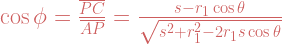
You can take this as a homework to prove that: $U(q_1,\,\vec{r}_1\,:\,q_2,\,\vec{r}_2) = k\frac{q_1q_2}{r_{12}}$ where r₁₂ is short notation for $\sqrt{r^2_1+r^2_2-2r_1r_2 \cos\theta}$ and therefore is the distance between the tip of r₁ and r₂, i.e. its the separation between r₁ and r₂, position vectors: in still simpler terms its the distance between the pair of charges q₁ and q₂.

+ To see how this is done click here (you can hide this by another click)

We have to prove that 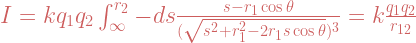$I=kq_1q_2\int_{\infty}^{r_2}-ds\frac{s-r_1\cos\theta}{(\sqrt{s^2+r^2_1-2r_1s \cos\theta})^3}=k\frac{q_1q_2}{r_{12}}$ . Lets assume $y=s^2+r^2_1-2r_1s \cos\theta$ , with this substitution: $dy = (2s - 2r_1\cos \theta)ds$ so that: $\frac{dy}{2} = (s - r_1\cos \theta)ds$ .

When s = ∞, y = ∞; when s = r₂, y = (r₁₂)², we have already mentioned that $r_{12}=\sqrt{r^2_1+r^2_2-2r_1r_2 \cos\theta}$ . Thus we have: $I=kq_1q_2\int_{\infty}^{r_{12}^2}\frac{(-\frac{1}{2})dy}{y^{\frac{3}{2}}}=kq_1q_2\frac{(-\frac{1}{2})y^{\frac{-1}{2}}}{(-\frac{1}{2})} \Big|_{\infty}^{r_{12}^2}=kq_1q_2\frac{1}{\sqrt{y}}\Big|_{\infty}^{r_{12}^2} =\frac{kq_1q_2}{r_{12}}$ . QED.

Electrostatic Potential Energy Of Many Pair Of Charges

Lets now generalize the above result we obtained to the case when there are more than 1 pair of charges in the configuration. Let charges q₁, q₂, q₃ … q_N be located at the positions given by position vectors r₁, r₂, r₃ … r_N.

Electrostatic Potential Energy Of 3 Discrete Charges

(3 × 2) / 2 = 3 Pairs Of Charge: For bringing charge q₃ to position specified by vector r₃, from ∞, when q₁ and q₂ are already present at r₁ and r₂ respectively, we use the superposition principle according to which: the total wok done in moving a 3rd charge in the combined field of two charges is the sum of the work done against the forces due to each of the two charges separately, i.e. in our notation of the potential energy: $U(q_1+q_2;\,\,\,q_3) = U(q_1,\,\vec{r}_1\,:\,q_3,\,\vec{r}_3) + U(q_2,\,\vec{r}_2\,: \,q_3,\, \vec{r}_3)$ .

So for a system of 3 charges for which there can be 3 pair of charges, the total potential energy of the configuration is the individual sum of potential energy for each pair, i.e. $U_3 = U(q_1,\,\vec{r}_1\,:\,q_2,\,\vec{r}_2) + U(q_1,\,\vec{r}_1\,:\,q_3,\,\vec{r}_3) + U(q_2,\,\vec{r}_2\,: \,q_3,\,\vec{r}_3)$ .

An alternative way to see this: we can also think of this as assembling the charges into its present configuration beginning with bringing the charges one by one, from ∞, to their respective positions. For the first charge there won’t be any work done. For the second charge the work done is what we calculated as potential energy of a pair of charge. The 3rd charge will experience force from each of the first two, as part of the pair it is considered in. So there are 3 pairs and each pair contribute according to the expression we first derived for the pair. viz. $U(q_a,\,\vec{r}_a\,:\,q_b,\,\vec{r}_b) = k\frac{q_aq_b}{r_{ab}}$

Electrostatic Potential Energy Of 4 Discrete Charges

(4 × 3) / 2 = 6 Pairs Of Charge: Similarly we can write the potential energy of 4 discrete charges q₁, q₂, q₃, q₄ at locations: r₁, r₂, r₃, r₄. There are now 6 pairs and the index i runs from 1 to 4 while index j runs from 2 to 5 respectively (i.e j = i + 1). The first particle comes to its position and no work is done. For the second particle the work done equals potential energy of the pair as derived above: this is the first pair. For the 3rd charge there are now two pairs formed with the first and the second charge: these are the 2nd and the 3rd pair. For the 4th charge there are 3 pairs with the 3 charges already brought in: these are the 4th, 5th and the 6th pair. Hence for the Nth charge there are always N – 1 pairs that are formed by the Nth charge with the N – 1 previously occupied charges. In concise indexed notation we write: $\boxed{U_4 = \sum_{\substack{i=1\\j=i+1} }^{\substack{j=i+1 \\ i=4}} U(q_i,\,\vec{r}_i\,:\,q_j,\,\vec{r}_j)}$ .

Electrostatic Potential Energy Of N Discrete Charges

(N × (N – 1)) / 2 Pairs Of Charge: Now we can easily generalize this to the case of the N discrete charge system, which as we mentioned consists of (N × (N – 1)) / 2 pairs with each pair of charge denoted by indices i and j has a distance of separation given by the magnitude of the separation vector r_ij: 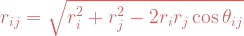$r_{ij}=\sqrt{r^2_i+r^2_j-2r_ir_j \cos\theta_{ij}}$ where $\cos\theta_{ij}=\hat{r}_i\cdot\hat{r}_j$ . So the potential energy of a N discrete charge configuration where the respective charges are at their respective positions (charges q₁, q₂, q₃ … q_N are located at the positions given by position vectors r₁, r₂, r₃ … r_N) is given by: $\boxed{U_N = \sum_{\substack{i=1 \\ j=i+1}}^{\substack{j=i+1 \\ i=N-1}} U(q_i,\,\vec{r}_i\, :\,q_j,\,\vec{r}_j)=\sum_{\substack{i=1\\ j=i+1}}^{\substack{j=i+1\\i=N-1}} k\frac{q_i q_j}{r_{ij}}}$ .

Alternative Ways to Express Potential Energy Of Electrostatic Configurations

Before we delve into our next interesting problem for calculating the electrostatic potential energy we will first show that there are several equivalent ways of representing the electrostatic potential energy.

Electrostatic Potential Energy of a Discrete Charge Configuration

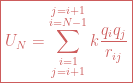
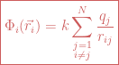
We have already seen above that for a discrete charge distribution with point charges q_i at positions given by vectors r_i, i = 1, 2, 3, …, N the total electrostatic potential energy is given by: $\boxed{U_N = \sum_{\substack{i=1\\ j=i+1}}^{\substack{j=i+1\\i=N-1}} k \frac{q_i q_j}{r_{ij}}}$ where r_ij is given by: $r_{ij}= \sqrt{r^2_i +r^2_j-2r_ir_j \cos\theta_{ij}}$ and $\cos\theta_{ij} =\hat{r}_i \cdot \hat{r}_j$ .

Electrostatic Potential Energy Of A Discrete Charge Configuration In Terms Of Potential

We now want to rewrite the electrostatic potential energy into an alternate form: 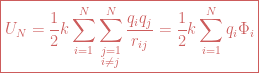$\boxed{U_N = \frac{1}{2}k \sum_{\substack{i=1}}^{\substack{N}} \sum_{\substack{j=1 \\ i\ne j}}^{\substack{N}} \frac{q_i q_j}{r_{ij}}=\frac{1}{2}k \sum_{\substack{i=1} }^{\substack{N}}q_i\Phi_i}$ with $\boxed{\Phi_i(\vec{r}_i)= k \sum_{\substack{j=1 \\ i\ne j}}^{\substack{N}} \frac{q_j}{r_{ij}}}$ , called the potential, which is produced by charges with index j except i and experienced by the charge with index i.

Electrostatic Potential Energy Of A Continuous Charge Configuration In Terms Of Potential

This can now be generalized to continuous charge distributions which are characterized by the volumetric charge distribution: $\rho(\vec{r})$ and we have the expression for potential energy in terms of potential by the expression: $\boxed{U=\frac{1}{2}\int \rho(\vec{r}) \Phi(\vec{r})d\tau}$ .

Electrostatic Potential Energy Of A Continuous Charge Configuration In Terms Of Electric Field

We can use vector identities (you can check some of them here) to recast the above expression for electrostatic potential energy into another relevant form, in terms of the electric field vector E, instead of the scalar field “potential” Φ that we have been dealing so far with.

Application of Gauss Divergence Theorem

We know that: $\boxed{\vec{\nabla} \cdot(f\vec{A})=f(\vec{\nabla}\cdot \vec{A}) +\vec{A}\cdot( \vec{\nabla}f)}$ . Now we will integrate this expression over a volume (whose infinitesimal element is dτ): $\int \vec{\nabla} \cdot(f\vec{A})d\tau = \int f(\vec{\nabla}\cdot \vec{A}) d\tau + \int \vec{A}\cdot( \vec{\nabla}f)d\tau$ . We can now convert the left hand side of the equation into a surface integral by using Gauss Divergence Theorem (The Gauss divergence theorem relates the flux of a vector field through a closed surface to the divergence of the field in the volume bounded by the surface, mathematically: $\int_V (\vec{\nabla}\cdot \vec{A})d\tau=\oint_S \vec{A}\cdot d\vec{S}$ ).

We have after this application: $\oint_S f\vec{A}\cdot d\vec{S}= \int f(\vec{\nabla}\cdot \vec{A}) d\tau + \int \vec{A}\cdot( \vec{\nabla}f)d\tau$ , with slight rearrangement: $\boxed{\int f(\vec{\nabla}\cdot \vec{A}) d\tau = -\int \vec{A}\cdot( \vec{\nabla}f)d\tau +\oint_S f\vec{A}\cdot d\vec{S}}$ .

Application of Gauss Law to convert Potential into Electric Field

We just mentioned above the form of the electrostatic potential energy for a continuous distribution in terms of potential: $U=\frac{1}{2}\int \rho(\vec{r}) \Phi(\vec{r}) d\tau$ and the volume charge density is given by Gauss Law (Gauss Law is discussed in detail here) $\rho=\epsilon_0 \vec{\nabla} \cdot \vec{E}$ . Using the second expression in the first: $U=\frac{\epsilon_0}{2}\int (\vec{\nabla} \cdot \vec{E}) \Phi d\tau$ .

In order to use the vector identity we established above (viz. $\int f(\vec{\nabla}\cdot \vec{A}) d\tau = -\int \vec{A}\cdot( \vec{\nabla}f)d\tau +\oint_S f\vec{A}\cdot d\vec{S}$ ) we recognize vector variables A = E and scalar functions f = Φ. With this the potential energy is now given as: $\frac{\epsilon_0}{2}\big[-\int \vec{A}\cdot( \vec{\nabla}f)d\tau +\oint_S f\vec{A}\cdot d\vec{S}\big]$ . But the electric field is the negative gradient of the potential: $\vec{\nabla}\Phi = -\vec{E}$ (worked out here in great detail). This leads to the following expression therefore for the potential energy: $U=\frac{\epsilon_0}{2}\big(\int_V E^2d\tau +\oint_S \Phi \vec{E}\cdot d\vec{S}\big)$ .

If we include all space for the integration (parts where there is no charge sources does not contribute) the first term is slated to increase with volume only (as integrand is a square term and is positive) this increase must be compensated by the decrease in the second term. The second term’s variation is ~ 1/r term, this can be seen from E → 1/r², dτ → r³, Φ → 1/r and dS → r² etc. Since we took volume V to be all space this means the bounding surface of this volume (which is S if you have been attentive all along) has a radius which is ∞.

Thus as we just understood the second term must go to zero at this limit. We are left with: $\boxed{U= \frac{\epsilon_0}{2}\int_{All space} E^2d\tau}$ . $u(\vec{r}) =\frac{\epsilon_0}{2} E^2$ is known as the energy density of the electrostatic field.

Electrostatic Potential Energy Of Uniform (Non-conducting) Spherical Charge Distribution

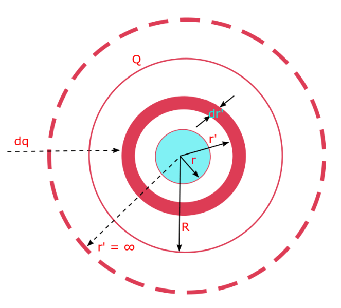
For calculating the potential energy of a sphere of charge distribution $\rho (\vec{r})$ we need to assemble shells with uniformly distributed charge from their initial position at ∞ to the desirable final position which can vary from radius r = 0 to r = R, R being the specified radius of the sphere of charge. Let us depict the situation by the following diagram.

Assembling a spherical charge distribution consists of bringing in shells of charge of radius r' that varies from infinity to a given comlplete radius starting from r=0 to r=R the given radius of the sphere of charge Q. — Assembling a spherical charge distribution consists of bringing in shells of charge of radius r’ that varies from infinity to a given complete radius starting from r=0 to r=R the given radius of the sphere of charge Q.

At any intermediate stage we have a sphere of radius r up-to which the desired sphere has been completed, and a shell of thickness dr’ and is brought from ∞ and located at r’. Thus this intermittent radius r’ has an initial value ∞ and final value r. The uniformly charged shell is outside of the sphere of radius r and experiences a field due to the charged sphere of radius r.

This field is given by: $\vec{E}(\vec{r}\,')=\big(\frac{4\pi}{3}\rho r^3\big)\frac{k}{{r\,'}^2}\hat{r}'$ . The points on the shell are moving along $-\hat{r}\,'$ . Charge on the shell = dq = 4πρr²dr. Work done (by external agent) in moving the shell a distance of dr’ (against the electrostatic force exerted by the charged sphere of radius r *) $dW(r, r\,')= dq \vec{E}\cdot (\hat{r}\,' dr\,')=4\pi \rho r^2 dr \frac{k4\pi\rho r^3}{3r\,'^2}dr\,'$ .

* Remember that its necessarily a repulsive force for the given configuration of spherical charge since we are building a uniform sphere where all charges are alike.
in general for calculation of potential or potential energy in other circumstances, it can be an attractive force as well

Total work done in bringing the shell from r’ = ∞ to r’ = r, against the repulsive electrostatic force of the charge already sitting in the sphere of radius r, is then given by: $dW(r)= k \frac{16}{3}\pi^2\rho^2 r^5 dr \int_{\substack{\\ \infty}}^{\substack{r}} \frac{dr\,'}{3r\,'^2}dr\,' =k \frac{16}{3}\pi^2\rho^2 r^4 dr$ .

We now continue building the sphere from r = 0 to r = R. For this the work done is given by integrating the last expression: $W(R) =\int_{\substack{\\ r=0}}^{\substack{r=R}} dW(r) = \int_{\substack{\\0}}^{\substack{R}} k \frac{16}{3}\pi^2\rho^2 r^4 dr =k \frac{16}{3}\pi^2\rho^2 \frac{R^5}{5} dr$ . But Q = (4πρR³)/3. Thus teh potential energy is determined to be: $\boxed{U_{sphere}=W(R) = \frac{3kQ^2}{5R}}$ .

Electrostatic Potential Energy Of Uniform Conducting Solid Sphere

Application: Compute the electrostatic energy of a conducting solid sphere of radius R and having total charge Q using the expressions for the electrostatic energy in terms of the electric field E of the above sphere.

For conductors electric field is zero if r < R. For r ≥ R, E = kQ/r² so $U= \frac{\epsilon_0}{2}k^2 Q^2 \int \frac{1}{r^4} d\tau$ . Its fairly easy and basic to evaluate this integral, so take this as a homework. We get the final expression for the electrostatic potential energy of a charged conducting sphere to be $U= \frac{k Q^2}{2R}$ which is identical for that of a spherical conducting shell as well. (Take $d\tau=r^2 \sin\theta d\theta d\phi$ , solid angle integration gives 4π). This makes sense since on a solid conducting sphere all charges reside on its surface which is equipotential, inside of it field is zero, contributing to no potential energy (this is the beauty of the potential energy expression in terms of square of electric field). Outside of it the shell and the solid sphere have same form for the potential as just given. Inside of the solid sphere the potential has to be constant (by integrating the zero electric field we obtain a constant).

There are several other configurations where we can calculate the potential and now we have multiple methods of doing so. Electrodynamics text of Griffith is a good source of such problems and multiple ways to solve these problems. There are a treasure trove of other excellent texts on electricity and magnetism.

Now its enough to hit the publish button I guess.

M Dash Foundation: C Cube Learning

Invariance: A journal with a difference, where mind meets aspiration

Electrostatic Potential Energy Of Different Charge Configurations. Lecture-10, 11.

Electrostatic Potential Energy Of A System Of Charge, A Charged Sphere And A Conducting Solid Sphere, Lecture-10, 11.

Definition Of Potential energy Of An Electrostatic Distribution Of Charges

Electrostatic Potential Energy Of A System Of Discrete Charge

Electrostatic Potential Energy Of A Pair Of Charge

Electrostatic Potential Energy Of Many Pair Of Charges

Electrostatic Potential Energy Of 3 Discrete Charges

Electrostatic Potential Energy Of 4 Discrete Charges

Electrostatic Potential Energy Of N Discrete Charges

Alternative Ways to Express Potential Energy Of Electrostatic Configurations

Electrostatic Potential Energy of a Discrete Charge Configuration

Electrostatic Potential Energy Of A Discrete Charge Configuration In Terms Of Potential

Electrostatic Potential Energy Of A Continuous Charge Configuration In Terms Of Potential

Electrostatic Potential Energy Of A Continuous Charge Configuration In Terms Of Electric Field

Application of Gauss Divergence Theorem

Application of Gauss Law to convert Potential into Electric Field

Electrostatic Potential Energy Of Uniform (Non-conducting) Spherical Charge Distribution

Electrostatic Potential Energy Of Uniform Conducting Solid Sphere

Leave a Reply Cancel reply

Electrostatic Potential Energy Of A System Of Charge, A Charged Sphere And A Conducting Solid Sphere, Lecture-10, 11.

Definition Of Potential energy Of An Electrostatic Distribution Of Charges

Electrostatic Potential Energy Of A System Of Discrete Charge

Electrostatic Potential Energy Of A Pair Of Charge

Electrostatic Potential Energy Of Many Pair Of Charges

Electrostatic Potential Energy Of 3 Discrete Charges

Electrostatic Potential Energy Of 4 Discrete Charges

Electrostatic Potential Energy Of N Discrete Charges

Alternative Ways to Express Potential Energy Of Electrostatic Configurations

Electrostatic Potential Energy of a Discrete Charge Configuration

Electrostatic Potential Energy Of A Discrete Charge Configuration In Terms Of Potential

Electrostatic Potential Energy Of A Continuous Charge Configuration In Terms Of Potential

Electrostatic Potential Energy Of A Continuous Charge Configuration In Terms Of Electric Field

Application of Gauss Divergence Theorem

Application of Gauss Law to convert Potential into Electric Field

Electrostatic Potential Energy Of Uniform (Non-conducting) Spherical Charge Distribution

Electrostatic Potential Energy Of Uniform Conducting Solid Sphere

Rate this:

Share this:

Like this:

Related

Leave a Reply Cancel reply