Electric Field and Gauss Law, Lecture 1

Lectures on Electricity and Magnetism — new series of lectures – EML – 1

All articles in this series will be found here. Click on link to left or search for menu “E AND M BASICS” on top.

Electric Field and Gauss Law

Electric Field

Electric field is the amount of Coulomb’s force, that a positive charge of 1 unit experiences at a given position. Its a vector in the same direction as that of the electric force, experienced by this unit charge. We will discuss the time independent electric field which is also known as the static field.

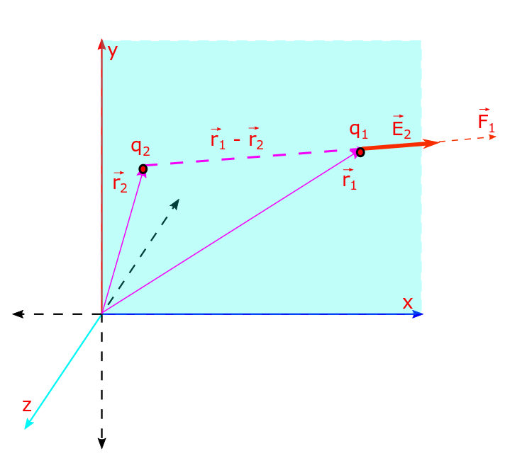
The Coulomb’s inverse square force law states that the force between two point charges q₁ located at a position r₁and q₂ located at a position r₂ is directly proportional to the product of the magnitude of the charges and inversely proportional to the square of distance of separation between the two charges. The direction of the force is given by the separation vector between the charges. The charges would experience a force which is directed along the line joining the position of the two charges. In other words its a central force. Its attractive for two unlike charges and repulsive between like charges.

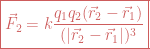
E.g. q₁ would experience a force given by: $\boxed{\vec{F}_1= k\frac{q_1 q_2 (\vec{r}_1-\vec{r}_2)}{(|\vec{r}_1-\vec{r}_2|)^3}}$ . Similarly q₂ would experience a force given by: $\boxed{\vec{F}_2= k\frac{q_1 q_2 (\vec{r}_2-\vec{r}_1)}{(|\vec{r}_2-\vec{r}_1|)^3}}$ . These two forces are an action-reaction pair and by Newton’s 3rd law are equal in magnitude and opposite in sign (i.e. in direction). This is a characteristic of the central force.

Newton’s 3rd law has two forms. According to the strong form, i.e. more restrictive form, in addition to being equal and opposite the forces are also directed along the line joining the two charges. The less restrictive form is known as weak form, and the forces are only equal and opposite but not along the line joining two objects exerting these forces, in that scenario, they are no more central forces. Coulomb’s law being a central force satisfies the strong form of Newtons 3rd law.

Magnetic forces are non-central forces and as such they do not obey Newton’s 3rd law (probably because Newton wasn’t a very magnetic persona) but its more appropriate to say that they do not obey strong form of Newton’s 3rd law, they do obey the weak form though.
This leads to non-conservation of angular momenta, which is fixed by some sort of unification.

Thus F₁ is the force exerted by q₂ and experienced by q₁. We define electric field as the force experienced by a unit charge, thus the electric field (vector) E₂ created by q₂ is the force experienced by q₁ divided by q₁. In other words E₂ = F₁/q₁ or F₁ = q₁E₂. Similarly F₂ = q₂E₁. The electric fields E₂ and E₁ are given by: $\boxed{\vec{E}_2= k\frac{q_2 (\vec{r}_1-\vec{r}_2)}{(|\vec{r}_1-\vec{r}_2|)^3}}$ and $\boxed{ \vec{E}_1 = k\frac{q_1 (\vec{r}_2-\vec{r}_1)}{(|\vec{r}_2-\vec{r}_1|)^3}}$ . Once we understand this much we won’t make a mistake with the vector formula F = q E, the E and F vector are produced by different charges (you can call them the source charge) and experienced by different charges (you can call them the reference charge).

Coulomb's Force Law and Coulomb's electric force and electric field: In the vector formula F = q E, the E and F vector are produced by different charges eg q2 (you can call them source charge) and experienced by different charges eg q1 (you can call them reference charge). — Coulomb’s Force Law and Coulomb’s electric force and electric field: In the vector formula F = q E, the E and F vector are produced by different charges eg q₂ (you can call them source charge) and experienced by different charges eg q₁ (you can call them reference charge).

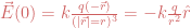
Now if the source charge (the one that produces the electric force or electric field), lets denote it by q₂ = Q, is located at r₂ = 0, i.e. the source is located at origin and the reference charge (the one that experiences the force or electric field), denoted by q₁ = q, is located at r₁ = r, then the electric fields are given by: 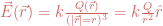$\vec{E}(\vec{r})= k\frac{Q (\vec{r})}{(|\vec{r}|=r)^3} = k\frac{Q}{r^2}\hat{r}$ and $\vec{E}(0) = k\frac{q (-\vec{r})}{(|\vec{r}|=r)^3} = -k\frac{q}{r^2}\hat{r}$ . So any charge Q produces an electric field at a distance r which is by the expression; $\boxed{\vec{E}(\vec{r}) = k\frac{Q}{r^2}\hat{r}}$ , where the unit vector is along the relative or separation position vector that begins at the source charge (here source point, location of Q) and ends at a point where we would like to determine the field (reference point, vector r). This is the Coulomb’s law expression for the electrostatic or electric field. The Coulomb’s force (on charge q) is now easy to express: $\boxed{\vec{F}(\vec{r}) = q\vec{E}(\vec{r}) = k\frac{qQ}{r^2}\hat{r}}$ . This is the Coulomb’s inverse square (force) law.

There is yet another useful notation scheme to present these expressions. The position vectors of the source charges is always denoted by the prime notation (eg vector r’) and the position vectors of the reference point (with or without a charge at this location) is denoted by unprimed notation (eg vector r). The separation vector r – r’ (note its always reference position minus source position, i.e. unprimed – primed) has a special notation: curly-r. It seems latex coding for this notation isn’t yet possible on this website. In HTML coding it looks like (reference is good but output isn’t completely accurate) 𝓇. So we would have to spell it out anytime we would like that notation scheme. In that scheme the electrostatic field is given by: 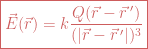$\boxed{ \vec{E}(\vec{r}) = k\frac{Q (\vec{r}-\vec{r}\,')}{(|\vec{r}-\vec{r}\,'|)^3}}$ . Its a generalized coordinate system scheme because we do not impose where origin would be and where charge source or reference points need to be. Just a convention that prime denotes source location.

Advantage of electric field

Advantage over electric force: Coulomb’s force law is a non-local expression, its a action-at-a-distance type quantity, i.e. the force is here at this instant and at any arbitrary distance apart at the same instant, it doesn’t get relayed, its instantaneous. This force which is supposed to transmit at infinite speed thus violates the special theory of relativity, where all speeds are bound by the limit of speed of light in free space. According to the postulate of this theory information can’t transmit faster than speed of light in vacuum. But field formulation is local, its compatible with special theory of relativity.
Electric fields are vector fields: there is a vector associated with every point in space and time. Once the field is known we don’t worry about nature of sources that produce these field. Physics becomes simpler as a consequence.

+ click to see more about this article

This article belongs to a group of lectures I intend to prepare for their online dissemination — these were delivered in a physical format, beginning with hand written notes that were delivered in a classroom full of students. This series is on Electricity and Magnetism and bears the name sake Electricity and Magnetism Lectures and the number of the lecture will be appended to the end to reflect the same. eg the current lecture will be named EML – 1 . This lecture was delivered to honors students on 30th Jan 2017.

In the meanwhile if you can’t wait and you need some of these concepts at the earliest, here is a slide-share presentation I had made roughly 5 years ago that consists of “some of the things” an undergrad needs: Electricity and Magnetism slides. There are other slides on different topics at that account of mine on slideshare.net (such as; Introduction to Quantum Mechanics , and these are quite well received by the community for their usefulness).

Electric field lines or lines of force

Since electric field is a vector field (you can see much detail regarding vector fields here) there is a vector associated with every point in space (in static situation we disregard time). Therefore we can draw the direction of the vector at each point in space. If direction vectors are drawn at close points we obtain continuous curves. The tangent to these curves represent direction of electric field at these points and the lines drawn with direction are known as “electric field lines or electric lines of force“.

Electric field lines and lines of force are synonymous, they are one and the same, but thats not true for magnetic field lines, they are always different from magnetic lines of force.
This is due to definition of magnetic field from Lorentz force which is a cross product of two vectors.

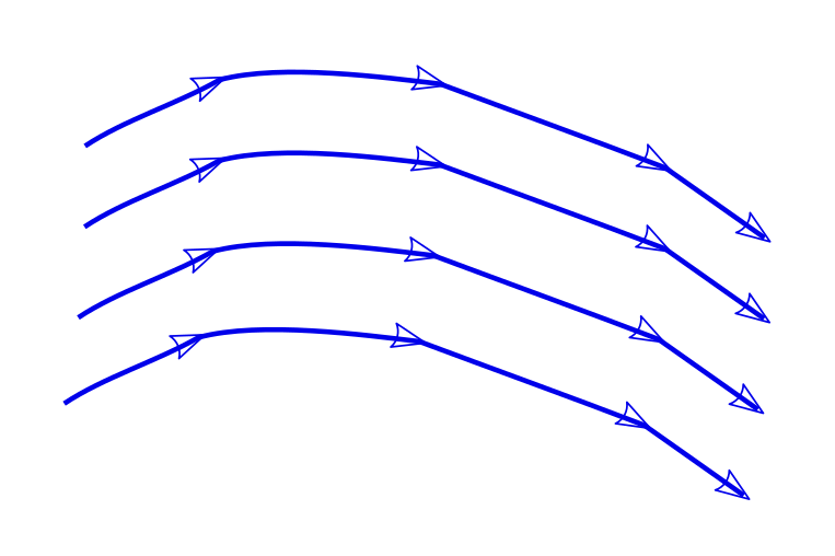
The following diagrams represent the lines of force for electric field created by a single positive charge, a single negative charge and an electric dipole.

lines of force for electric field created by a single positive charge and a single negative charge

lines of force for electric field created by an electric dipole

Nature of electric lines of force

The electric field due to point charges are very large (in magnitude) and are radially outward for +ve charges or radially inward for -ve charges. See diagrams above. Other charges can not produce such patterns of lines of force. So presence of such patterns of radial lines of force is a signature of point charges.
Electric lines of force tells us the direction of electric field at any point.
Density of electric field lines gives the relative magnitude of electric field (strength). High density means large electric field strength.

Electric flux

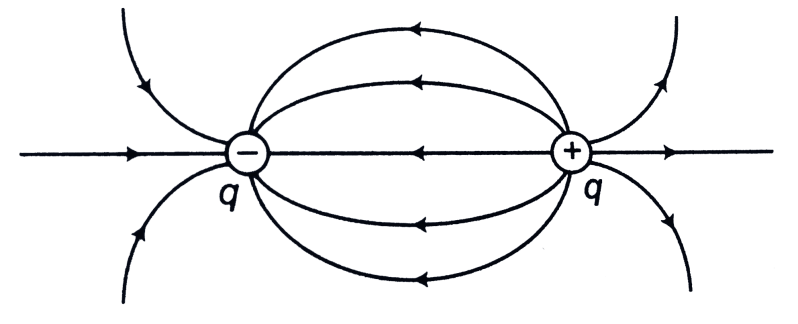
If electric field E is present in a region of infinitesimal area element dA then the electric flux is defined as $\boxed{d\phi_E=\vec{E}\cdot d\vec{A}=\vec{E}\cdot \hat{n}dA}$ . Here the unit vector n is defined as the normal to the surface area dA. For closed surface we are not free to define whether the surface has a positive or negative n. For example for a spherical surface n is always outward.

Flux is defined through normal to a surface and any vector that passes through the surface

For a large surface (i.e. one which isn’t uniform like an infinitesimal one) we need to integrate over all elements of the surface to find the flux.

The total outward flux across a closed surface due to charges present outside of it is zero. This is because as much flux enters the surface, as exits.
Flux would accumulate inside of a closed surface only if net charge accumulates.

Gauss Law

Consider a +ve point charge q at the center of a spherical surface S of radius R.

Positive charge q at the center of a sphere of radius R.

The electric field E due to the charge q is given by Coulomb’s law: $\vec{E}=k\frac{q}{R^2}\hat{r}$ . The area of the sphere is 4πR². The field E and the outward normal to the surface S are along the same direction: this gives dot product between E and normal vector n = magnitude of E. Thus total outward flux is given by: $\phi=k\frac{q}{R^2} \cdot 4\pi R^2 =4\pi kq$ . But this result is valid for surface of any shape.

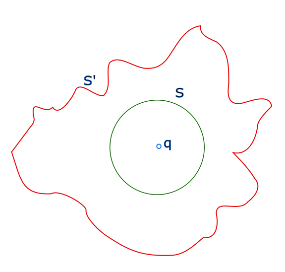
Lets consider two surfaces S and S’ as shown in the following diagram, S’ has an arbitrary shape, S is spherical. The flux due to q at the surface of S is -Φ = – 4πkq, since outward normal to S is towards q. But for the region inside S’ and S there is no charge. We just learned that if there is no charge enclosed in a surface then total flux is zero, So, outward flux of S’ must be +Φ.

The flux passing through a surface does not depend upon its shape but the total charge contained in it.

So Gauss law can be stated in the following form; total outward electric flux across any closed surface enclosing a charge Q is Φ = 4πkQ. Gauss law can be used with symmetry to evaluate unknown electric fields in many situations.

Illustration of Gauss Law with spherical symmetry

Calculate the electric field due to an uniformly charged sphere of radius R carrying a charge Q at a point P situated at a distance r > R, from its center.

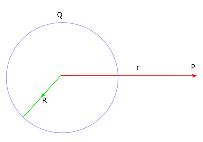
Spherical symmetry and Gauss Law. A uniformly distributed charged sphere and its field at an outside point can be calculated using Gauss Law.

Due to spherical symmetry the field at point P is unchanged if we rotate the sphere about the radial line. Lets denote this field as E(r) since it depends only on radial position r and not the azimuthal angle coordinate φ or polar angle wrt zenith coordinate θ.

Φ = E(r) × area of the spherical surface = 4πr²E(r), but flux is given by Gauss law as; flux = Φ = 4πkQ. So 4πr²E(r) = 4πkQ. Thus the field is given as E(r) = kQ/r². This is same as the field that would be produced at that point P, by a point charge, located at the center of the sphere.

M Dash Foundation: C Cube Learning

Invariance: A journal with a difference, where mind meets aspiration

Electric Field and Gauss Law, Lecture 1

Electric Field and Gauss Law