Application of matrix method to thick lens

This article is 3301 worded

Optics series, lecture — VI

This lecture was delivered on 7th February 2017 ( 1.5 hours )

( All Optics series lectures ) Read other available lectures in optics series

“Application of matrix method to thick lenses”

Application of matrix method to thick lens: cardinal points, thick and thin lens matrices, unit and nodal planes and more …

Matrix method for thick lens: the lens is the most important component of a an optical system. A ray is the most basic description of a light wave under geometric optics conditions. This is a representative image of the same. Photo Credit: mdashf.org — **Matrix method for thick lens**: the lens is the most important component of a an optical system. A ray is the most basic description of a light wave under geometric optics conditions. This is a representative image of the same. **Photo Credit**: mdashf.org

Topics covered in this lecture
A. Cardinal points
B. Thick lens equation and matrix for thick lens
C. System matrix for thin lens
D. Unit and Nodal planes
E. Matrix for a system of 2 thin lenses

Background

In our last lecture ( lecture V ) we introduced the matrix methods for optical systems. I recommend you read that lecture, preferably before the current one.

( matrix formulation in geometrical optics ) Read previous lecture ( lecture V ) on matrix method

Our previous studies of the optical systems were based on two premises.

a. we assumed a paraxial system

b. we assumed that our lenses are thin.

Paraxial system: We assumed a paraxial system. This means we employed a first order optical theory. Read more about paraxial systems and what is first order optical theory in the two lectures linked below. The paraxial assumptions are fraught with various types of aberrations. We studied about aberrations in quite detail in two lectures.
Thin lenses: We assumed that our lenses are thin. This we did for simplicity. In physics when we assume a simple situation, we are not evading the actual complexity of the situation, we are just postponing this to the happy hour, howsoever one defines it.

( Introduction to aberration ) Read an introduction to aberration and details of chromatic aberration

( Details about primary aberration ) Read details about primary or Seidel aberration

Happy Hours. Some people go by the Friday happy hour rule. It gives a good substratum on which a disposition can be carried out. Later one develops the nuances and fits it into the substratum and if things are carried out with caution and skill one gets a very effective overview of the pedagogy.

Let us now delve into the complexity of the optical system, as a next step from its simple substratum of a thin lens. Our previous analyses especially the ones we applied on the introductory lecture of matrix method ( lecture V ) needs to be modified for application to optical systems when we consider thick lenses.

In our last lecture, lecture — V, we studied the method of matrices in understanding optical ray tracing. Let us now apply this method to the case of the thick lens and see what power it unleashes.

( lecture – V: matrix formulation ) Read previous lecture on matrix method

Thick lens

I. Cardinal points

A thick lens can be considered to be an equivalent of multiple thin lenses.
Let us draw two suitable thick lens diagrams.

Matrix method for thick lens: Primary principal plane and cardinal points: The thick lens which is a lens of general nature can be studied efficiently by definition of what are called cardinal points. There are 6 cardinal points for an optical system like a thick lens. They are all defined in this diagram. This image starts with the primary principal plane and the first focal point in order to define the cardinal points. Photo Credit: mdashf.org — **Matrix method for thick lens**: Primary principal plane and cardinal points: The thick lens which is a lens of general nature can be studied efficiently by definition of what are called cardinal points. There are 6 cardinal points for an optical system like a thick lens. Some of them are defined in this diagram. This image begins with the primary principal plane and the first focal point in order to define the cardinal points. **Photo Credit**: mdashf.org

Matrix method for thick lens: secondary principal plane and cardinal points; The thick lens which is a lens of general nature can be studied efficiently by definition of what are called cardinal points. There are 6 cardinal points for an optical system like a thick lens. Some of them are defined in this diagram. This image shows the secondary principal plane and the second focal point in order to define the cardinal points. Photo Credit: mdashf.org — **Matrix method for thick lens**: secondary principal plane and cardinal points; The thick lens which is a lens of general nature can be studied efficiently by definition of what are called cardinal points. There are 6 cardinal points for an optical system like a thick lens. Some of them are defined in this diagram. This image shows the secondary principal plane and the second focal point in order to define the cardinal points. **Photo Credit**: mdashf.org

Let’s first discuss the parameters of the thick lens system.

First focal point or object focus: The first focal point ( FFP ) or object focus is denoted as $F_o$ . Check the first diagram above: rays emerging from $F_o$ , incident on the first spherical surface, will emerge parallel to the optical axis.
Second focal point or image focus: The second focal point ( SFP ) or image focus is denoted as $F_i$ . Check the second diagram above: if rays incident on the first spherical surface are parallel, then they meet at $F_i$ after refraction from second spherical surface.
The forward focal length: The forward focal length ( FFL ) is the distance between the object focus $F_o$ and the vertex to the first spherical surface, $V_1$ .
The backward focal length, B.F.L.: The backward focal length ( BFL ) is the distance between the image focus $F_i$ and the vertex to the second spherical surface, $V_2$ .
Image surfaces: When rays from the object and image focuses ( $F_o$ and $F_i$ ), are extrapolated they meet on a curved surface ( or line ), rather than a plane ( or a straight line ). Such a locus of points can also lie outside of the lens. The surface coincides with the principal planes in the paraxial region, — see principal planes below.
The principal planes: These planes are tangent to the surface which is created when rays from $F_o$ and $F_i$ are extrapolated. The principal planes meet the optical axis at 1st and 2nd principal points $H_1$ and $H_2$ .
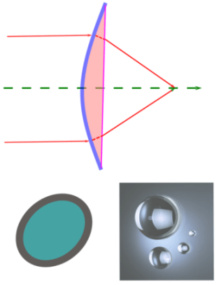
Nodal points: Any ray going through the optical center emerges parallel to the incident ray — see the diagram below. When the incident ray and the emergent rays are extrapolated they meet at points $N_1$ and $N_2$ on the optical axis. $N_1$ is called as the first nodal point and $N_2$ is called as the second nodal point. When the lens is surrounded by the same medium on both sides — and of-course has a symmetric geometry, then the nodal and the principal points are the same.

The six points that we just discussed, the focal points $F_o$ and $F_i$ , the principal points $H_1$ and $H_2$ and the nodal points $N_1$ and $N_2$ , are together known as cardinal points of the system.

The length between $H_1$ and $H_2$ is nearly equal to $\frac{1}{3}\,rd$ of the length between $V_1$ and $V_2$ for ordinary glass lenses in air.

Matrix method, thick lens: The nodal points N-1 and N-2 of the thick lens are defined from the incident ray, emergent ray and the optical axis, in this diagram. Photo Credit: mdashf.org — **Matrix method, thick lens**: The nodal points N-1 and N-2 of the thick lens are defined from the incident ray, emergent ray and the optical axis, in this diagram. **Photo Credit**: mdashf.org

II. Thick lens equations

Thick lenses are equivalent to two spherical refracting surfaces separated by a distance $d_1$ between the vertices. We can write a relation between the image distance $v$ , the object distance $u$ and the focal length $f$ , for a thick lens as follows given that; object distance $u$ is measured from the first principal plane $H_1$ and the image distance $v$ is measured from the second principal plane $H_2$ : $\boxed{\frac{1}{u}+ \frac{1}{v}=\frac{1}{f}}$

We would also have after a detailed considerations of the geometry the following relation which is valid for a thick lens. Alternatively we will derive the following result from our elegant and powerful matrix method, that we learned in last lecture, lecture — V: $\boxed{\frac{1}{f}= (n_l -1) \Big [ \frac{1}{R_1}-\frac{1}{R_2}+\frac{(n_l -1)d_l}{n_lR_1R_2}\Big]}$

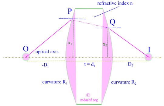
III. Setting matrix equation for thick lens

1. System matrix for thick lens

Its a cupcake to realize how to draw the paraxial ray diagram for a thick lens system, now that we understood in good detail how we can do it for a general traversal of the light ray in terms of translation and refraction, in lecture V, already linked twice. ( this will be the last time I promise )

( lecture – V: matrix formulation ) Read previous lecture on matrix method

So lets just do that. It will be easier to talk as analytical a topic as geometrical optics, when we have a geometrical diagram for it. Lets therefore draw one.

Matrix method for thick lens: Matrix transformation of the ray coordinate of a thick lens; the ray coordinates are an important parameter for description of optical systems under the assumption of geometrical or ray optics. How does the coordinate transform under various optical phenomena like reflection and refraction is important in understanding and predicting various optical phenomena. The matrix method gives a powerful and useful way for achieving this. Photo Credit: mdashf.org — **Matrix method for thick lens**: Matrix transformation of the ray coordinate of a thick lens; the ray coordinates are an important parameter for the description of optical systems under the assumption of geometrical or ray optics. How does the coordinate transform under various optical phenomena like reflection and refraction is important in understanding and predicting various optical phenomena. The matrix method gives a powerful and useful way for achieving this. **Photo Credit**: mdashf.org

Let the ray incident on the lens, strike the first surface at P with coordinates $(\lambda_1,\,x_1)$ and emerge at Q with coordinates $(\lambda_2,\,x_2)$ where $\lambda_1$ and $\lambda_2$ are the optical direction cosines as we defined in lecture — V.

As we can easily see the ray undergoes two refractions — one at P and one at Q, and one translation through thickness $t$ , from P to Q — with a paraxial assumption in the medium, with refractive index $n$ .

Accordingly: $\begin{pmatrix}\lambda_2 \\ x_2 \end{pmatrix}= \begin{pmatrix}1 & -P_2 \\ 0 & 1 \end{pmatrix} \begin{pmatrix}1 & 0 \\ \frac{t}{n} & 1 \end{pmatrix}\begin{pmatrix}1 & -P_1 \\ 0 & 1 \end{pmatrix} \begin{pmatrix}\lambda_1 \\ x_1 \end{pmatrix}$

With $P_1 = \frac{n-1}{R_1}, \,\,P_2 = -\Big (\frac{n-1}{R_2} \Big )= \frac{1-n}{R_2}$ we have the system matrix for a thick lens.

$\boxed{S=\begin{pmatrix} b & -a\\ -d & c \end{pmatrix} = \begin{pmatrix} 1- \frac{P_2t}{n}&-P_1-P_2 \big[ 1-\frac {tP_1}{n} \big ] \\ \frac{t}{n} & 1- \frac{t}{n}P_1\end{pmatrix}}$

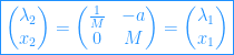
2. System matrix for thin lens as a limiting case of thick lens

For a thin lens we can safely assume the limiting thick lens whose thickness goes to zero: $t \to 0$ . This way — by approximating it from the thick lens, we do not lose any generality, that we would lose if a thin lens were to be considered a priori with the condition: $t \to 0$ .

We obtain: $\boxed{S=\begin{pmatrix} 1 & -P_1-P_2 \\ 0 & 1\end{pmatrix}}$

So, we have: $a = P_1 + P_2,\,\,\, b = c = 1, \,\,\,d = 0$ .

Now if we have $x_1 = 0$ then $x_2$ has to be zero as well. Thats because an image has to be axial, for an axial object point.

So we have $\boxed{bD_2 + aD_1D_2 - cD_1 - d = 0, \,\,\,or\,\,\, D_2 + (P_1 + P_2)D_1D_2 - D_1 = 0}$ .

This implies: $\boxed{\frac{1}{D_2} - \frac{1}{D_1} = P_1 + P_2 = (n-1)\Big (\frac {1}{R_1}-\frac {1}{R_2} \Big )}$

or $\frac{1}{D_2} - \frac{1}{D_1}= \frac{1}{f}, with \,\,\, f = \frac{1}{P_1 + P_2 }= \Big [ (n-1)\Big (\frac {1}{R_1}-\frac {1}{R_2} \Big ) \Big ]^{-1}$

Thus we see that the element $a$ in the system matrix is nothing but the inverse of the focal length or power of a lens. We get for thin lens the matrix: $\boxed{\begin{pmatrix} 1 & -\frac {1}{f} \\ 0 & 1\end{pmatrix}}$

Also we realize that the power of matrix method is such that we obtain the thin lens equation without even realizing, we did.

$\boxed{\frac{1}{f} = (n-1)\Big (\frac {1}{R_1}-\frac {1}{R_2} \Big )}$

Its so effortless.

3. Unit and nodal planes of thick lens from system matrix elements

The elements of the system matrix for a thick lens were obtained in the penultimate section. Lets open the system matrix $S$ that we obtained for a thick lens, and write down these elements one by one.

$\boxed{a = P_1 + P_2 \Big ( 1- \frac {t}{n}P_1 \Big ) \,\,\,\,\,\, b= 1 - \frac {t}{n} P_2 \,\, \,\,\,\,\,\, c= 1 - \frac {t}{n} P_1\,\,\,\,\,\, \,\,d= -\frac {t}{n}}$

A. Unit planes

The locus of conjugate points — object and image that is, for which linear magnification is unity ( = 1 ) are called as unit planes. These are also the principal planes that we defined at the beginning of this article, while discussing cardinal points.

A paraxial ray emanating from unit plane in object space will emerge at the same height in image space in the other unit plane. If $d_{u1} = 0$ and $d_{u2} = 0$ represent distances of unit planes from refracting surfaces then: $\boxed{b+ad_{u1}=\frac {1}{c-ad_{u2}}= 1}$

We note that we would obtain the above result after an equally enlightening analysis of a thick lens system, as we did here and the analysis in lecture — V.

Earlier I intended this as a homework for the serious student, but below I have worked this out, nonetheless one who works this out himself/herself will no doubt reward himself/herself conceptually and spiritually.

Here is how to obtain the above result. Multiply the system matrix that we obtained for thick lens, namely $S$ , with a translation matrix $T_1$ on left and a translation matrix $T_2$ on right, in terms of distances $- D_1$ and $D_2$ respectively, as we have seen these are the distances measured from the usual vertices $V_1$ and $V_2$ — and the refractive index of air is $n_{air}=1$ .

We would obtain: $\boxed{\begin{pmatrix} \lambda_2\\x_2 \end{pmatrix} = \begin{pmatrix} b+aD_1 &-a\\ bD_2 + aD_1D_2-cD_1-d & \,\,\,\,\,\,\,\,\,c-aD_2\end{pmatrix} =\begin{pmatrix} \lambda_1\\x_1 \end{pmatrix}}$

Note that all that we did here is from our original system matrix $S$ we obtained a new system matrix. The old system matrix $S$ gave the traversal of ray from its coordinate of incidence at the first surface, to the coordinate of ray incidence at the second surface.

But before incidence at point P — that is: the first surface, the ray had traversed from the object point — this is given by matrix $T_1$ through a translation of distance $D_1$ and after incidence at point Q — that is at the second surface, the ray would traverse to image point — this is given by matrix $T_1$ through a translation of distance $D_1$ .

So including these two additional coordinates changed the old system matrix $S$ to this new one above. Now let us apply two conditions. One of the conditions we have already used in our lecture today.

a. Condition — i: Axial object points produce axial image points.

That is: $x_1 = 0$ means $x_2=0$ . We would get a relationship between $D_1$ and $D_2$ , namely: $\boxed{bD_2 + aD_1D_2-cD_1-d =0}$

This was one of the elements of the matrix we just obtained above, this is the beauty of the matrix method, we obtain important results in terms of the elements of the system matrix. This implies, for the image plane, we obtain the equation:

$\boxed{\begin{pmatrix} \lambda_2 \\ x_2 \end{pmatrix} = \begin{pmatrix} b+aD_1 & -a \\ 0 & c-aD_2 \end{pmatrix} = \begin{pmatrix} \lambda_1 \\ x_1 \end{pmatrix}}$

Now we apply the second condition.

b. Condition — ii: If our objects points are not axial we get: $x_2 = (c - aD_2) x_1$ . So magnification of the system is $M = \frac{x_2}{x_1} = c - aD_2$ . The system matrix obtained above should be unitary, that is, its determinant should be unity ( = 1 ).

This gives us what we set out to prove, with the recognition that M = 1 in our case, because we are fixed to the unit planes, the ones that have linear magnification by definition, namely: $\boxed{b+ad_{u1}=\frac {1}{c-ad_{u2}}= \frac{1}{M} = 1}$

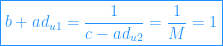
and we have a general result: $\boxed{\begin{pmatrix} \lambda_2 \\ x_2 \end{pmatrix} = \begin{pmatrix} \frac{1}{M} & -a \\ 0 & M \end{pmatrix} = \begin{pmatrix} \lambda_1 \\ x_1 \end{pmatrix}}$

Now the distances of the unit planes — the primary plane to vertex $V_1$ distance: $d_{u1}$ and the secondary plane to vertex $V_2$ distance: $d_{u2}$ can be solved in terms of system matrix elements.

We have: $\boxed{d_{u1}=\frac{1-b}{a}, \,\,d_{u2}=\frac{c-1}{a}}$

If S is the distance of the object plane from first unit plane and v is the distance of the image plane from second unit plane then; $D_1 = u+d_{u1}=u+\frac{1-b}{a}, \,\,\,D_2 = v+d_{u2}=v+\frac{c-1}{a}$ , applying condition — i, that is: $bD_2 + aD_1D_2-cD_1-d =0$ and taking 3^rd and 4^th term to the RHS, $D_2 = \frac{d+cD_1}{b+aD_1} \,\,\,det \,S =bc-ad=1$ .

So we have: $\boxed{\frac{1}{v}- \frac{1}{u}=a}$ — take this as a homework to prove this from above.

In section — II for thick lens we saw that instead of a we had the inverse of focal length — the left hand side is equal if we consider the minus sign for sign convention. So the matrix element again gives the inverse of focal length, as in case of thin lens, which we had seen before. Thus $\frac{1}{a}$ is the focal length of an optical system if distances are measured from unit planes.

Thus for thick lens we have the locations of the unit planes: $\boxed{d_{u1}=\frac{t}{n}{P_2} {\Big [P_1+P_2\Big ( 1-\frac{t}{n}P_1 \Big) \Big]}^{-1} }$ and $\boxed{d_{u2}=-\frac{t}{n}{P_1}{\Big [P_1+P_2\Big ( 1-\frac{t}{n}P_1 \Big) \Big]}^{-1}}$

For symmetric thick-lens: $\boxed{d_{u1}=\frac{t}{2n} }$ , $\boxed{d_{u2}=-\frac{t}{2n}}$ and $\boxed{\frac{1}{f}=a = P_1 + P_2 \Big ( 1- \frac{t}{n}P_1\Big) =(n-1)\Bigg [ \frac{1}{R_1}-\frac{1}{R_2}+\frac{(n-1)t}{nR_1R_2}\Bigg]}$

This is exactly what we had stated in the beginning of our article in section — II. We see that we can obtain the fundamental equations of thick lens and thin lens almost effortlessly if we are to follow the magic of matrix method.

B. Nodal planes

We apply similar reasoning to obtain the nodal plane distances. By using our condition — ii

$\boxed{\begin{pmatrix} \lambda_2 \\ x_2 \end{pmatrix} = \begin{pmatrix} b+aD_1 & -a \\ 0 & c-aD_2 \end{pmatrix} = \begin{pmatrix} \lambda_1 \\ x_1 \end{pmatrix}}$

we see that; $\boxed{d_{n1}=\frac{1-b}{a} = d_{u1}}$

this is because the media on both sides of the lens is air and also the lens is symmetric. We had stated this earlier, now we have evidence.

Similarly second nodal plane is same as second unit plane. So: $\boxed{d_{n2}= \frac{c-1}{a} = d_{u2}}$

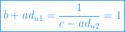
4. System of two thin lenses from system matrix elements of thick lens

If two thin lenses of focal lengths $f_1$ and $f_2$ are considered then the system matrix is easy to guess based on our discussion above; a is the inverse of focal length. The distance of separation between them is simply a translation of thickness t.

We have, $\boxed{S = \begin{pmatrix}1 & -\frac{1}{f_2} \\ 0 & 1 \end{pmatrix} \begin{pmatrix}1 & 0 \\ t & 1 \end{pmatrix}\begin{pmatrix}1 & -\frac{1}{f_1} \\ 0 & 1 \end{pmatrix}}$ which yields the matrix elements: $\boxed{a=\frac{1}{f_1}+\frac{1}{f_2}-\frac{t}{f_1f_2}, \,\,\,\,\,\,\,\, b=1-\frac{t}{f_2}, \,\,\,\,\,\,\,\, c=1-\frac{t}{f_1}, \,\,\,\,\,\,\,\, d = -t}$ and we have $\boxed{a=\frac{1}{f}=\frac{1}{f_1}+\frac{1}{f_2}-\frac{t}{f_1f_2}}$

This is the result we had used in studying achromatic doublets, when we studied chromatic aberrations.

( Achromatic doublets ) Read about achromatic doublets in the linked lecture

Also the unit planes are located at $\boxed{d_{u1}=\frac{1-b}{a}=\frac{tf}{f_2}\, \, \, \, \, \, \, \, \, \, \, \, d_{u2}=\frac{c-1}{a}=-\frac{tf}{f_1}}$ .

5. System of two thin lenses: Ramsden and Huygens’s eyepieces

This is merely an application of section – 4 above. I leave this to your good sense for trying this as a homework problem and get some conceptual clarity on the differences between the two types of eye pieces.

One thought

Pingback: Harmonic Spherical Waves « Invariance Publishing House

M Dash Foundation: C Cube Learning

Invariance: A journal with a difference, where mind meets aspiration

Application of matrix method to thick lens