The Bohr model of the Hydrogen atom: atomic spectra and quantization, Quantum Lecture – 4 and 5.

Lectures on Quantum Mechanics — new series of lectures – QL- 4 & 5.

All articles in this series will be found here. Click on link to left or just search for menu “Quantum Lectures” on top.

The Bohr model of the Hydrogen atom: atomic spectra and quantization.

+ click to see more about this article

This article belongs to a group of lectures I intend to prepare for their online dissemination — without prior preparation to be delivered in a physical format, such as a hand written note to be delivered in a classroom full of students. This series is on quantum mechanics and bears the name sake Quantum Lectures and the number of the lecture will be appended to the end to reflect the same. eg the current two lectures will be named QL – 4 & 5.

In the meanwhile if you can’t wait and you need some quantum concepts at the earliest, here are two slide-share presentations I had made roughly 5 years ago that consists of most of “some of the things” an undergrad needs along with some solved problems from Griffith’s introductory text on quantum mechanics: quantum slides 1, quantum slides 2. There are other slides on different topics at that account of mine on slideshare.net (such as electromagnetic waves, and these are quite well received by the community for their usefulness).

The emission spectra of elements.

Light and color

Light is known to have possessed various colors. It would be more appropriate to state that light and color are two entirely distinct entities. Light does not contain color just like you do not contain your spouse. Its another matter you both appear at the same venue on the basis of the same invitation card. Its Newton who first realized this. He proclaimed thus: light is the physical phenomena and color is the sensation our eyes produce of it.

You must have known about Pit Vipers (pythons and boas as well), the deadly snakes that detect infrared radiation, which is a particular type of light (bam, heat is transmitted as light) thats devoid therefore of the properties of visibility but only in terms of color. The viper nonetheless is capable of biting us in the tenebrous moonless nights sensing the infrared signal our body would exude in that darkness. Different humans are capable of sensing different colors of the same light wavelength? At-least thats what I have come across in some social media images. Hence color is merely a detector effect.

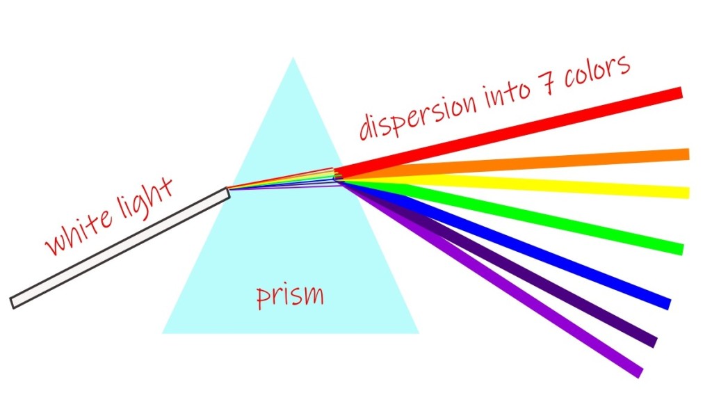
Dispersion: resolving light into its components

Newton was a weird fellow, who pierced his own eyes with a sharp object to study its optical properties apart from threatening his parents to shut them in a room and set the room on pyre. But his physics was right. It was he who first resolved white light into its component colors (as we just learned more correct would be to say into its component wavelengths) by the help of a prism which acts on the mechanism of dispersion.

Emission and Absorption lines

Decades later it was Melvill who evidenced that light from an incandescent gas consists of discrete value of wavelengths. These are known as emission lines as they appear as lines on a photographic plate owing to their discrete nature. Thus emission line spectra is observed in one of these two cases

• An electric discharge passes through a gas
• A volatile salt is put into a flame

When a light that consists of a continuous spectrum is irradiated on atoms the process exhibits an absorption line spectra. When e.g. white light is incident on the absorbing layers of an atomic element and the resultant spectrum is analysed with the help of a spectrograph the photographic plate is darkened everywhere except for several unexposed lines. These lines correspond to the discrete values of wavelengths that were absorbed by the atoms in the absorbing layer.

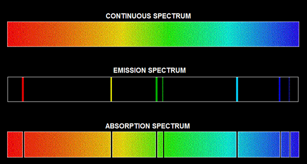
In 1859, Kirchhoff evidenced that lines for wavelengths of absorption coincide with the same for wavelengths of emission, for the atoms of the same element, and each element has its own unique signature of line spectrum for emission and absorption. You can see the first fact in the diagram appended above. The characteristic lines of spectrum of any element is a great tool in recognizing the presence of the element in a chemical analysis or astrophysical study for cosmic objects.

Balmer Series

In 1885, J. Balmer stumbled upon a certain regularity in the pattern of the line spectra of hydrogen atom. Finding regularities and pattern is one of the chief aims of scientists, it helps them refine the status of knowledge and make further progress possible. Balmer found the eponymous line spectrum known as the Balmer Series which is shown in the following diagram.

This series consists of visible and near ultraviolet wavelengths and these are named in a particular manner by assigning the Greek subscripts α, β and γ etc to the sequence of lines. The lines are more and more closely spaced when the wavelengths they represent decreases. There is a limit to this series of lines of the hydrogen atom at a wavelength of 3646 Å. The 9 known lines at the time then satisfied the following formulaic expression: λ = Cn²/(n² – 4). Here the constant C equals to 3646 Å and n is an integer that takes the values: 3 for α, 4 for β, 5 for γ, 6 for δ and so on depicting the lines H_α, H_β, H_γ etc in the Balmer line spectrum.

Balmer-Rydberg formula and further series of hydrogen atom

4 years later J.R. Rydberg found that the lines of the Balmer series can as well be stated in terms of the wave number ν (same as the inverse of the wavelength λ, i.e. ν = 1/λ) and these are given by: . Here n stands for integer values larger than 2 and R_H is the Rydberg constant with a value of 109 677.58 cm^-1 obtained experimentally. This equation (can be called as Balmer-Rydberg formula now) can be generalized to accommodate subsequent findings of ultraviolet and infrared spectra of the hydrogen atom. where n_a = 1, 2, … and n_b = 2, 3, … and n_b is always larger than n_a. ν_ab is the wave number of either an absorption line or emission line.

There are many series now. n_a = 1 and n_b = 2, 3, … is known as Lyman series and its an ultraviolet spectrum. n_a = 2 and n_b = 3, 4, … is known as Balmer series that we just discussed. n_a = 3, 4, 5 and n_b = n_a+1, n_a+2 etc are known as Paschen, Brackett and Pfund series respectively and all 3 are infrared spectrum. In the same way for Balmer series the lines in each series are labelled by the Greek subscripts: α, β, γ and δ etc for increasing values of wave number.

Ritz combination principle.

Each of the terms in the Balmer-Rydberg formula is called a spectral term. Thus: ν_ab = T_a – T_b, with T_a = R_H/n_a² and T_b = R_H/n_b². Atoms other than hydrogen can have their own spectral terms except the form of expression for these terms might be more complicated than the above. Since the wave number of any line of emission or absorption is a difference of two spectral terms, a set of spectral terms define the atomic spectra and collectively these are known as the term system of the atom. This generalization was achieved by W. Ritz. When 3 wave numbers (of 3 spectral lines) are represented by 3 terms: ν_ij = T_i – T_j, ν_jk = T_j – T_k, ν_ik = T_i – T_k we can write: ν_ik = (T_i – T_j) + (T_j – T_k) = ν_ij + ν_jk. The addition of wave number this way, states an example of the Ritz combination principle.

It was Niels Bohr who first gave the partially successful explanation of the regularities in the emission and absorption line spectrum — only for the hydrogen atom or hydrogen like “atoms” (1 electron bound to a nucleus or an ion). This was 1913 and Bohr used the new ideas of Planck’s and Einstein’s quantum concepts and the experimental results about the nuclear atom, by Rutherford, Geiger and Marsden.

Rutherford’s model of the nucleus and the atom.

It was Rutherford who had famously studied the behavior of the atom by the alpha-particle scattering experiment. Alpha particles are helium atoms which have shed two of their electrons. The target was a thin metallic foil (Gold). The results were startling to say the least. The initial discovery was a collaboration between Rutherford, Geiger and Marsden. The probe particles were supposed to be deflected only a very little under the elastic Coulomb scattering. But 1 in roughly 8000 of them suffered massive deflections (larger than 90⁰ scattering angle).

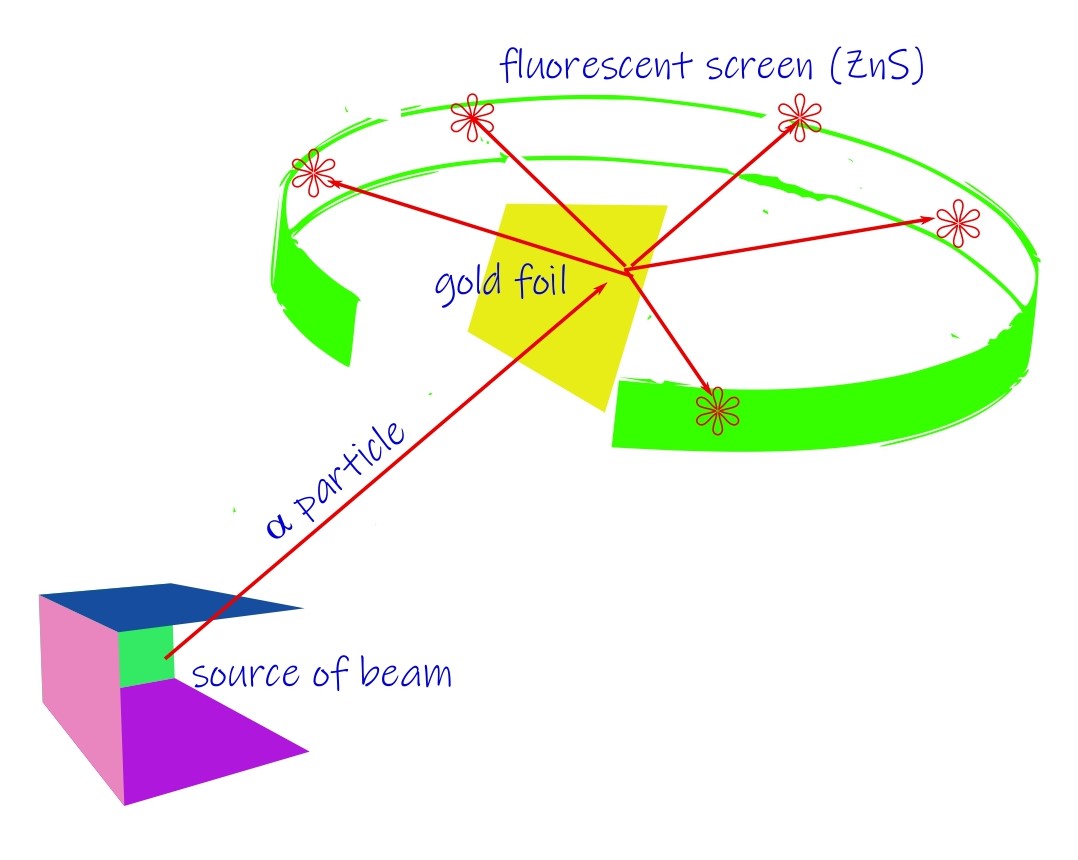
By 1911, the inference Rutherford drew from this was that the atom consists of a dense mass at the center where all the positive charges are concentrated. It was called the nucleus. The size of the nucleus was determined to be at-least of the order of 10^-14 m or smaller while the atomic size comes to 10^-10 m. The experimental evidence came quite swiftly (by 1913) and Rutherford model was held to be an accurate model of reality. But there was the topic of stability of such an atom. A planetary model was chosen where the negatively charged electrons would revolve around the positive core named the nucleus. But this wasn’t enough. It was known from classical physics of electromagnetism that an accelerated charge must radiate away its energy. If that were so, the electron in the Rutherford’s model would need to collapse within 100 ps, a really small time. But this is contrary to what happens in reality, atoms are greatly stable.

Bohr’s model of the hydrogen atom.

Bohr took a clue from all the great ideas that were put forth previously, Planck’s quantum of energy (see here), Einstein’s photon as the quantum of electromagnetic field (see here) and Rutherford’s nucleus in the atom as a core and electrons revolving in a planetary orbits. In these orbits the electrons experience the electrostatic Coulomb’s force and for simplicity he considered the orbits to be circular rather than the general elliptical orbits allowed in classical mechanics.

Stationary energy states

Like Planck Bohr hypothesized a revolutionary idea: that of stationary states. Only a specific number of orbits can be assumed by the electrons in orbital motion. These allowed orbits have their associated energy and thus are called allowed energy levels. Lets denote these orbits by the value of their energy: E_a, E_b, E_c … etc. He further postulated that as long as the electrons are in these stationary states they do not radiate electromagnetic energy.

Transition between energy states

But radiation of electromagnetic energy occurs when there is a transition between different orbits. The difference in the energy value then, between any two energy levels or stationary states gives the frequency of the photon which is to be emitted. In symbols: hν = E_b – E_a where E_b must be greater in value than E_a for emission of radiation. This frequency-energy relation is known as Bohr’s frequency relation.

Another energy unit

In accordance with this relation energy can often be expressed either in eV units or in Hz as well as cm^-1 units (based on energy, frequency and wave number units for energy). 1 eV ≡ 2.41797 × 10¹⁴ Hz ≡ 8065.48 cm^-1. This relation also implies that the spectroscopic terms that we already discussed are nothing but energy values of various allowed energy levels or stationary states.

Quantization of angular momenta

Bohr continued on the path of quantization (he didn’t stop at an ad-hoc hypothesis of energy quantization, he invented yet another, like we don’t stop at one excuse, we invent more and more) for the 1-electron hydrogen atom. By quantizing the magnitude of the orbital angular momentum of the electron in its stationary orbit around the hydrogen nucleus, he achieved the quantization of energy. The angular momentum L takes on only those values that satisfy: L = nh/2π = nℏ where n is a quantum number thats a positive integer i.e. n = 1, 2, 3, … and ℏ is the reduced Planck’s constant. This then lends credence to how energy is quantized for an electron in a bound state with the nucleus of the hydrogen atom. We will now see how.

Let us assume an infinitely heavy nucleus so that its essentially at rest in comparison to the electron’s revolution around it. This is a temporary restriction that we can lift later to see how that can impact our result. But this is the simplest thing to do in this situation. We also assume that the electron moves at essentially non-relativistic speed v in circular orbits of radius r. Its the Coulomb’s attractive force between the electron and the nucleus of charge Ze which provides for the centripetal acceleration of the electron’s circular motion. Hence we can write: 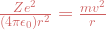. Bohr’s postulate on the quantization of angular momentum then provides for another equation: L = mvr = nℏ.

Stationary states are quantized energy levels

From the last two expressions we see that its the speed and radius of the electron itself which are quantized. They are given by: and . The kinetic energy can now be given: . Total energy E is the sum total of the kinetic energy and the potential energy, and we can set our total energy to be zero (E = 0) when the electron is at rest (v = 0, so T = 0) and completely separated from the nucleus (r = ∞ this means n = ∞ and again v is zero). In essence that means both kinetic energy T and potential energy V are zero at infinite separation and hence total energy is. Thats because the Coulomb’s potential energy is given by: , this means potential energy is also quantized and given by: . This gives us the quantized expression for the total energy of the bound state of the electron and the nucleus. Thus the allowed energy levels or stationary states are given by: with n = 1, 2, 3 … etc.

Naming of quantized energy states

Thus the energies of the bound states of 1 electron atoms are discrete. The integer n is called the principal quantum number. The lowest energy state is known as the ground state and its given by the quantum number n = 1. The higher energy states given by are known as excited state, with increasing n as first excited state (n = 2) second excited state (n = 3) and so on. The excited energy values converge to the value of zero when n goes to ∞. The ground state is known as K shell, similarly the first excited state is known as L shell and second as M shell, and so on.

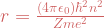
Energy level diagrams of the hydrogen atom. (and the likes)

In an energy level diagram energy is plotted in the vertical-axis and energy levels are drawn on the horizontal axis. The following figure shows the energy level diagram of the hydrogen atom, as per the predicted values from Bohr’s model. There are two energy scales that are shown on the plot, on the left in terms of wave number (cm^-1) and on the right in terms of energy in electron volt.

The Rydberg constant in Bohr’s theory

Now that we know the energies of various levels, in the hydrogen atom, we can relate pairs of them to the frequency of light emitted when the electron makes a transition between them. So if the pairs of levels are denoted by E_a and E_b, then the frequency is given by: where the pairs of quantum numbers associated with their energy level by their subscript are related as: n_b > n_a. By denoting: and setting Z = 1 for the atomic hydrogen entities, we obtain the wave number expression, exactly in the same form and function as that given in the Balmer-Rydberg formula that we have had our first (and successive for the fanboy) assignation with. The infinite sign should not scare you or your neophyte friends from non-physics background (with a superficial interest in Physics, may be just a fad that fades away) it merely signifies one of our assumption, that the infinite-some mass of the nucleus (which takes away the burden of extra motion) has been in stead. We are not really fat-shaming the nucleus: its capable of some real motion. But we will switch on our camera only when we are math-ready.

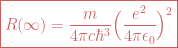
The above expression thus opens up a vista where we have one more way to predict the value of the Rydberg constant and vet it out with the experimental decree of the same. The Bohr’s theory gives us the Rydberg constant in terms of the fundamental constants and it turns out to be: 109737 cm^-1, its good but not in perfect consonance with the experimental value that we have mentioned earlier.

Ionization energy and bound state vs free states

Lets rewrite the quantized energy levels in this way: E_n = -I_P/n², where . A positive amount of energy -E_n = I_P/n² is needed to ionize the electron in its nth orbit. When the electron is in its ground state this positive energy is known as the ionization potential of the atom. In our infinite nuclear mass approximation this is just I_P. In photo-ionization the atom absorbs a sufficiently high energetic photon and emancipates the incarcerated electron into the land of positive energy, the promised land of freedom. Collision processes are also capable of dislodging electrons by imparting them the ionization energy.

Positive energy of a system of nucleus and electron signifies the system is unbound. Positive energies are not discrete but arbitrarily continuous. As a comprehensive description transitions can occur between bound and bound states which projects a discrete energy spectrum, between bound and a free state projecting a discrete-continuous spectrum and finally between a free and free state projecting a continuous-continuous variation in the energy spectrum.

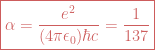
The fine structure constant in Bohr’s theory: radius and velocity of electron in the ground state

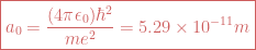
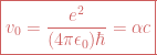
The radius of the electron in the ground state of the hydrogen atom is known as the first Bohr radius or colloquially the Bohr radius. Its denoted by: a₀. Its obtained from the general expression for radius by setting Z = 1 and n = 1. Thus . In a similar fashion the electron velocity in the ground state is given by: . The dimensionless constant α is known as “fine structure constant“: .

The non-relativistic nature of the Hydrogen atom problem

v₀ ≈ αc = c/137. Thus we see that the velocity of the electron in the ground state is 137 times slower compared to the speed of light in free space, — velocity decreases when we go further up to the excited states. This explains why Bohr’s non-relativistic assumption of electron’s velocity is right on the money. Now we can rewrite the quantized energy in terms of fine structure constant, and we obtain: . Thus when Z is not too large the absolute value of the total energy (the binding energy i.e. |En|) is small compared to the rest mass energy of the electron, mc². This is yet another tell-tale sign of the non-relativistic nature of the hydrogen atom as studied by Bohr.

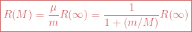
Finite nuclear mass.

What would happen to all that we have arrived at if suddenly the nucleus wishes to dance? We can no longer say to it “hey look, stop being funny, you are infinitely heavy”. The actual nucleus has a finite mass and if we take this into account we need to accommodate this in some way. There is a nice way to achieve this. Its called the reduced mass thing in the two body problem. Now the center-of-mass does not lie inside of nucleus but somewhere between the nucleus and the electron. To our calculations it wouldn’t matter as long as the center of mass is at rest or in uniform motion. Its definitely not being accelerated would be our excuse if somebody extends his logical course of interrogations with the famous “what if”. But as honest as we physicists are this is true only if there are no external forces acting on the system of the nucleus and electron.

The reduced mass approach

So the electron mass is m and nucleus mass is M, you said? Thats all we need to incorporate into our analysis. We now introduce our most beloved thespian, the angular momentum in its more refined attires, the reduced mass μ = mM/(m+M), L = μvr. The Bohr’s angular momentum quantization condition is now altered to suit the new situation: L = μvr = nℏ. The kinetic energy of the system is simply: T = μv²/2. Potential energy remains same as its not a function of masses (but positions of those masses wrt each other hence only radius, and of-course the charge the masses possess.)

Modified values of energy, radius and Rydberg’s constant

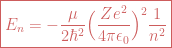
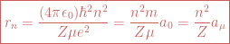
For getting the expressions for quantized energy and radius we only need to replace the mass m by the reduced mass μ. We get: and where a_μ = (m/μ)a₀ is the modified Bohr radius. With the correction to the nuclear mass the Rydberg constant is now calculated to be: . For atomic hydrogen its the proton which is the nucleus, as a result M is replaced by proton mass M_P and the Bohr’s value for Rydberg’s constant becomes 109681 cm^-1 and this agrees to the experimental value mentioned earlier to better than 40 parts per million.

Consequence of finite mass

There are 2 immediate consequences of the fact that the nuclear mass is finite as we have incorporated this into the body of our analysis.

• A. All the frequencies of the spectral lines of 1 electron atoms are now reduced by the factor: wrt the value calculated with infinite mass approximation. Thus different isotopes will have different frequencies for the same line without the correction. This frequency shift is how deuterium (the heavier twin of hydrogen) was discovered.
• B. The second consequence is due to atom’s recoil when it emits (or absorbs a photon). Let P be the magnitude of the momentum of the atom which is initially at rest, after recoil from emitting a photon of energy hν. Then due to conservation of momentum: P = hν/c. The kinetic energy of the recoiled atom is now P²/2M = (hν)²/2Mc², where M is the mass of the atom (essentially same as nuclear mass). The conservation of energy yields the relation: Δν_R/ν = ± hν/2Mc² where Δν = ν – ν₀, ν₀ being the frequency without mass correction. Here the + sign corresponds to absorption and – for emission. This effect is very small, since the fractional frequency shift is easily seen to be of the order of 10^-9. But it implies emission and absorption are no more identical. Which means emitted radiation by an atom can’t be absorbed by the same atom, as before, evidenced by Kirchhoff. This also goes against experimental evidence. This apparent paradox is taken care of by the Heisenberg’s uncertainty principle.

Limitations of Bohr’s model

This model is successful in explaining the energy levels of 1-electron atoms but leaves a lot to be wanted.

• Its a hybrid theory incorporating classical ideas and new ones that are contradistinction to the old: classical theory. eg the problem of the stability of the atom has a stopgap provision that the electron won’t radiate while its in one of the stationary orbit.
• The quantization of the angular momentum is an ad hoc proposition.
• Only circular orbits being proposed as the orbit is arbitrary.
• Can not deal with systems with more than 1 electron.
• No reliable method to compute rate of transition between different levels.
• Can’t describe the unbound systems.

Conclusion

Sommerfeld and Wilson later showed how restrictions of circular orbits can be removed. Sommerfeld obtained relativistic corrections to the Bohr’s model. But its woes persisted eventually it was superseded by rigorous quantum mechanical theories developed by Schrodinger, Heisenberg, de Broglie and Dirac et al.

What remains in this article is a few lines on the Bohr Correspondence principle and if possible the detailed description on Frank Hertz experiment. I will do the first anon, but still debating whether to make the second a lecture on its own or not. For now though this article is swollen enough to go into the online world, in its 2 lecture format. Do follow up with your comments or doubts etc.